ECON 4910 Spring 2007 Environmental Economics Lecture 9

ECON 4910 Spring 2007 Environmental Economics Lecture 9: Stock pollution Perman et al. Chapter 16 Lecturer: Finn R. Førsund Stock pollution 1

Effects of pollution n Two ways q q n Environmental effects of pollution within a time period as function of pollutants discharged during the same period Environmental effects within a time periods a function of accumulated amounts of pollutants from earlier periods The time dimension of accumulation effects q q Real time: accumulation over short time periods, e. g. accumulation of organic waste over a few hours in a river, important when ecosystems are highly vulnerable to extreme values in real time, threshold values for when “bad things” happen, e. g. day variation in oxygen in rivers Discrete time with longer time periods, day, week , month , year: total load is the determining the pollution effect, not variation within the chosen time period, e. g. death of fish when snow melts in spring with accumulated acidity. Stock pollution 2

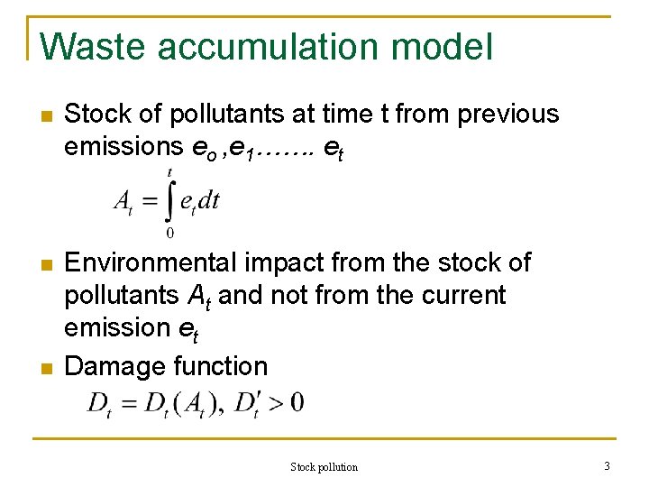
Waste accumulation model n Stock of pollutants at time t from previous emissions eo , e 1……. et n Environmental impact from the stock of pollutants At and not from the current emission et Damage function n Stock pollution 3

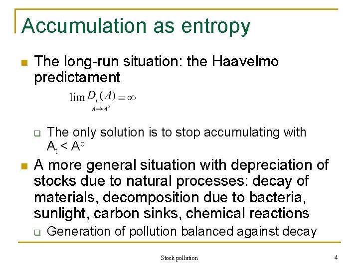
Accumulation as entropy n The long-run situation: the Haavelmo predictament q n The only solution is to stop accumulating with At < Ao A more general situation with depreciation of stocks due to natural processes: decay of materials, decomposition due to bacteria, sunlight, carbon sinks, chemical reactions q Generation of pollution balanced against decay Stock pollution 4

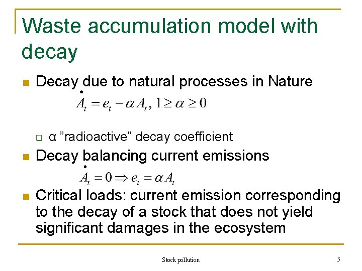
Waste accumulation model with decay n Decay due to natural processes in Nature q α ”radioactive” decay coefficient n Decay balancing current emissions n Critical loads: current emission corresponding to the decay of a stock that does not yield significant damages in the ecosystem Stock pollution 5

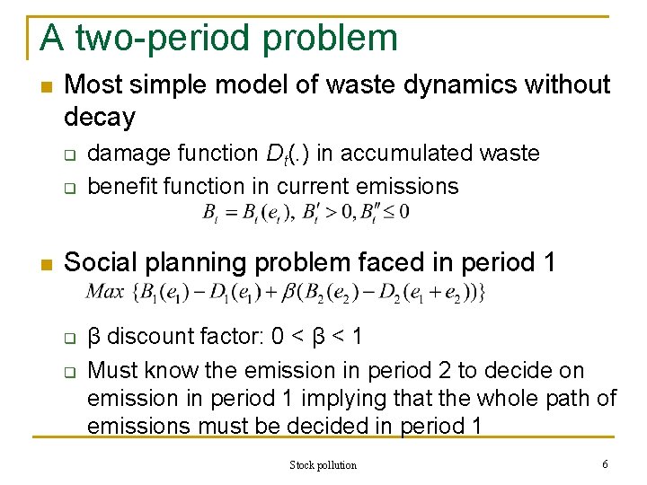
A two-period problem n Most simple model of waste dynamics without decay q q n damage function Dt(. ) in accumulated waste benefit function in current emissions Social planning problem faced in period 1 q q β discount factor: 0 < β < 1 Must know the emission in period 2 to decide on emission in period 1 implying that the whole path of emissions must be decided in period 1 Stock pollution 6

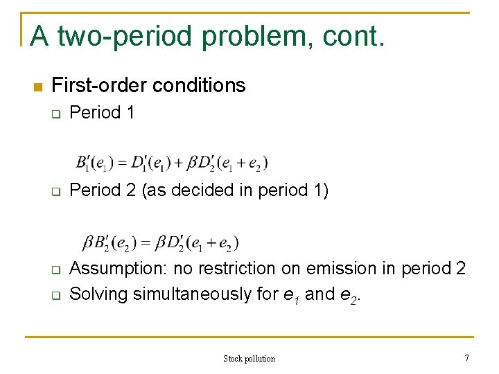
A two-period problem, cont. n First-order conditions q Period 1 q Period 2 (as decided in period 1) q q Assumption: no restriction on emission in period 2 Solving simultaneously for e 1 and e 2. Stock pollution 7

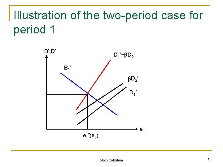
Illustration of the two-period case for period 1 B’, D’ D 1’+βD 2’ B 1’ βD 2’ D 1 ’ e 1*(e 2) Stock pollution 8

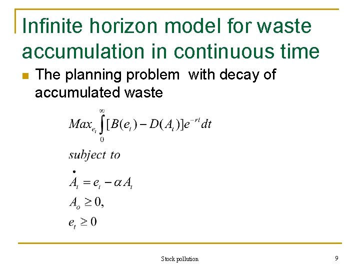
Infinite horizon model for waste accumulation in continuous time n The planning problem with decay of accumulated waste Stock pollution 9

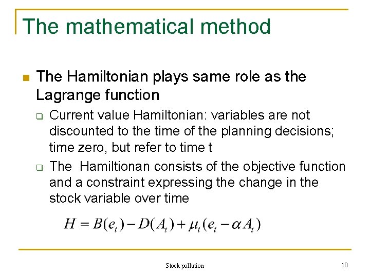
The mathematical method n The Hamiltonian plays same role as the Lagrange function q q Current value Hamiltonian: variables are not discounted to the time of the planning decisions; time zero, but refer to time t The Hamiltionan consists of the objective function and a constraint expressing the change in the stock variable over time Stock pollution 10

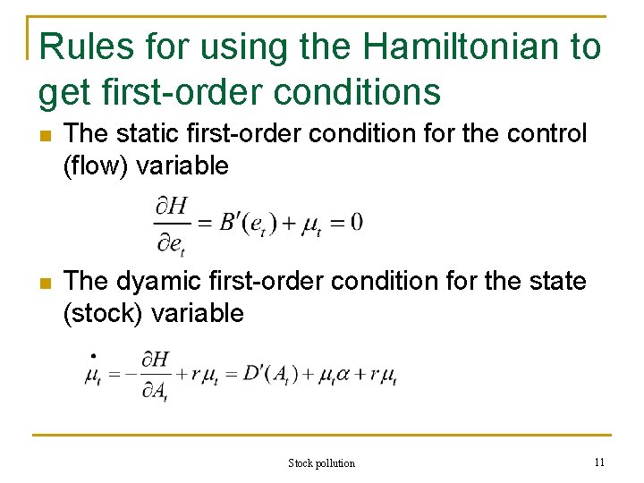
Rules for using the Hamiltonian to get first-order conditions n The static first-order condition for the control (flow) variable n The dyamic first-order condition for the state (stock) variable Stock pollution 11

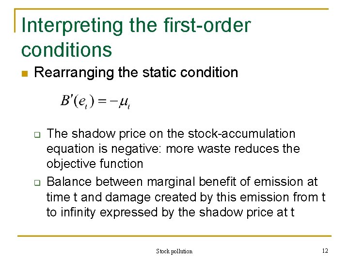
Interpreting the first-order conditions n Rearranging the static condition q q The shadow price on the stock-accumulation equation is negative: more waste reduces the objective function Balance between marginal benefit of emission at time t and damage created by this emission from t to infinity expressed by the shadow price at t Stock pollution 12

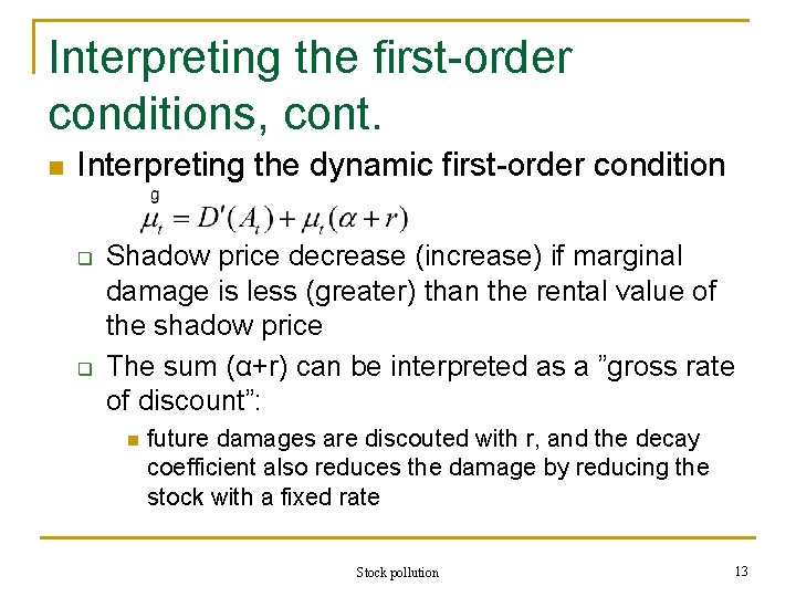
Interpreting the first-order conditions, cont. n Interpreting the dynamic first-order condition q q Shadow price decrease (increase) if marginal damage is less (greater) than the rental value of the shadow price The sum (α+r) can be interpreted as a ”gross rate of discount”: n future damages are discouted with r, and the decay coefficient also reduces the damage by reducing the stock with a fixed rate Stock pollution 13

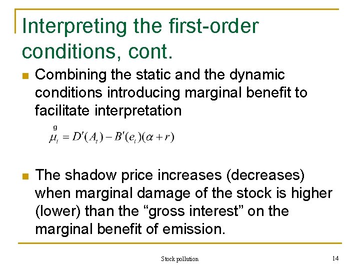
Interpreting the first-order conditions, cont. n Combining the static and the dynamic conditions introducing marginal benefit to facilitate interpretation n The shadow price increases (decreases) when marginal damage of the stock is higher (lower) than the “gross interest” on the marginal benefit of emission. Stock pollution 14

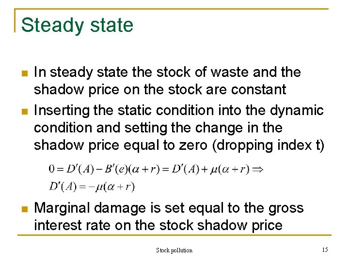
Steady state n n n In steady state the stock of waste and the shadow price on the stock are constant Inserting the static condition into the dynamic condition and setting the change in the shadow price equal to zero (dropping index t) Marginal damage is set equal to the gross interest rate on the stock shadow price Stock pollution 15

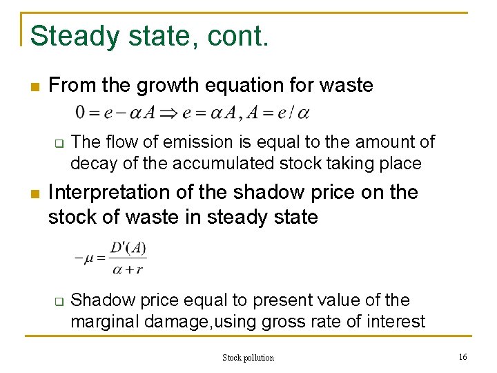
Steady state, cont. n From the growth equation for waste q n The flow of emission is equal to the amount of decay of the accumulated stock taking place Interpretation of the shadow price on the stock of waste in steady state q Shadow price equal to present value of the marginal damage, using gross rate of interest Stock pollution 16

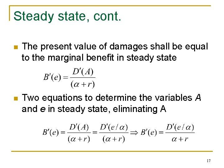
Steady state, cont. n The present value of damages shall be equal to the marginal benefit in steady state n Two equations to determine the variables A and e in steady state, eliminating A 17

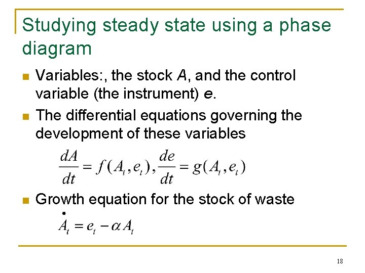
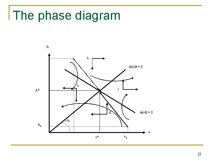
Studying steady state using a phase diagram n n n Variables: , the stock A, and the control variable (the instrument) e. The differential equations governing the development of these variables Growth equation for the stock of waste 18

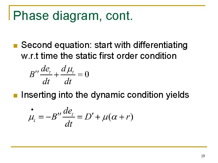
Phase diagram, cont. n Second equation: start with differentiating w. r. t time the static first order condition n Inserting into the dynamic condition yields 19

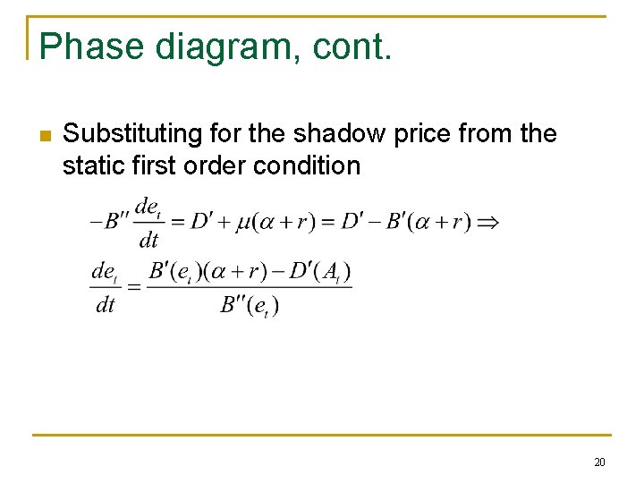
Phase diagram, cont. n Substituting for the shadow price from the static first order condition 20

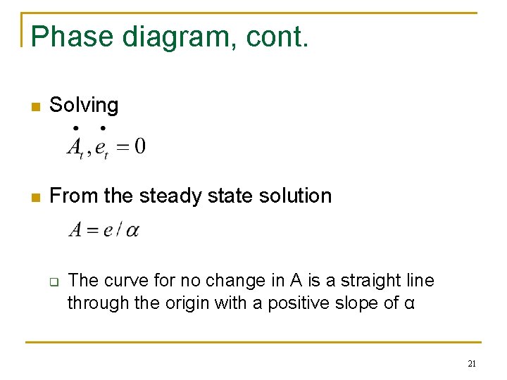
Phase diagram, cont. n Solving n From the steady state solution q The curve for no change in A is a straight line through the origin with a positive slope of α 21

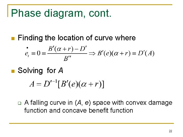
Phase diagram, cont. n Finding the location of curve where n Solving for A q A falling curve in (A, e) space with convex damage function and concave benefit function 22

The phase diagram A b d. A/dt = 0 a c A* d de/dt = 0 1/α Ao e e* eo 23