ECON 211 ELEMENTS OF ECONOMICS I Session 6

ECON 211 ELEMENTS OF ECONOMICS I Session 6– Production and Costs (Part 2) Lecturer: Dr. (Mrs. ) Nkechi S. Owoo, Department of Economics Contact Information: nowoo@ug. edu. gh College of Education School of Continuing and Distance Education 2014/2015 – 2016/2017

Session Overview • This session discusses a variety of other cost concepts useful for the analysis that follows, including totals (total cost, total variable cost, total fixed cost), averages (average total cost, average variable cost, average fixed cost), marginal cost, among others. • We long run cost concepts in this session. Slide 2

Session Outline The key topics to be covered in the session are as follows: • Production and Costs in the Long-Run • The relationship between Long-run and Short-run costs • Explaining the Shape of the LRATC curve – Economies of Scale – Diseconomies of Scale Slide 3

Reading List • Hall and Lieberman – Chapter 5 : pp: 174 - 182 Slide 4

Topic One PRODUCTION AND COSTS IN THE LONG RUN Slide 5

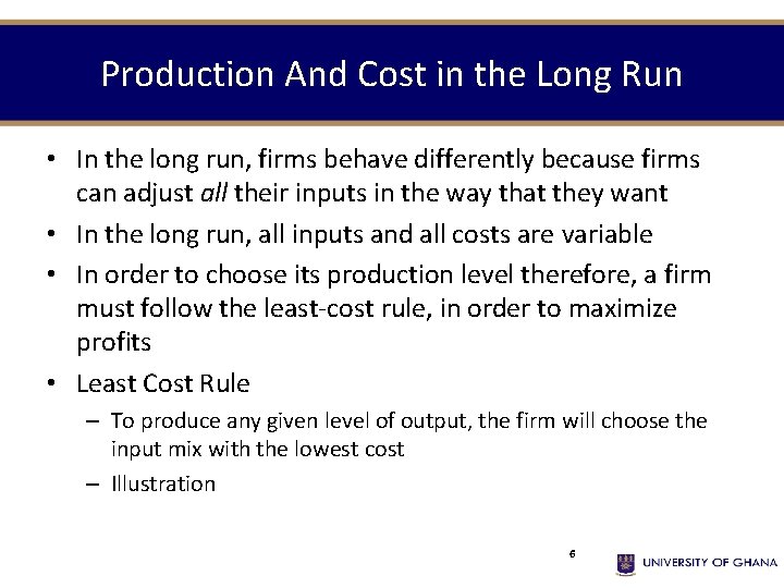
Production And Cost in the Long Run • In the long run, firms behave differently because firms can adjust all their inputs in the way that they want • In the long run, all inputs and all costs are variable • In order to choose its production level therefore, a firm must follow the least-cost rule, in order to maximize profits • Least Cost Rule – To produce any given level of output, the firm will choose the input mix with the lowest cost – Illustration 6

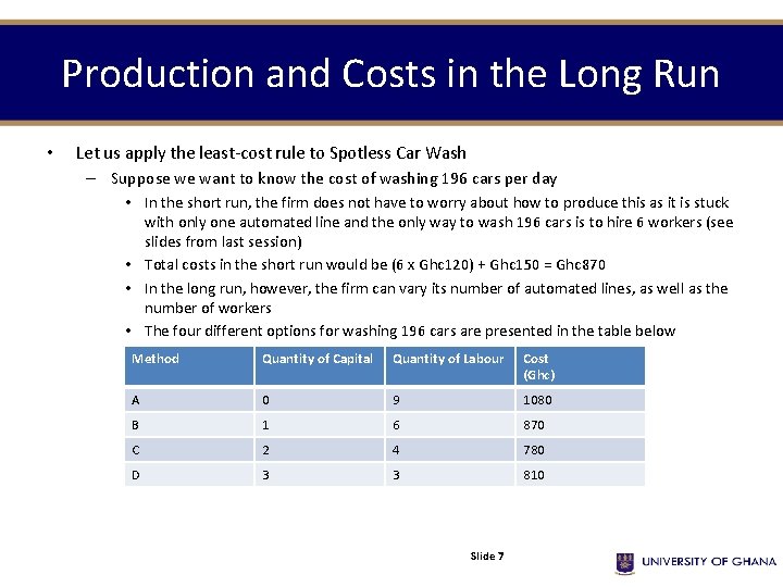
Production and Costs in the Long Run • Let us apply the least-cost rule to Spotless Car Wash – Suppose we want to know the cost of washing 196 cars per day • In the short run, the firm does not have to worry about how to produce this as it is stuck with only one automated line and the only way to wash 196 cars is to hire 6 workers (see slides from last session) • Total costs in the short run would be (6 x Ghc 120) + Ghc 150 = Ghc 870 • In the long run, however, the firm can vary its number of automated lines, as well as the number of workers • The four different options for washing 196 cars are presented in the table below Method Quantity of Capital Quantity of Labour Cost (Ghc) A 0 9 1080 B 1 6 870 C 2 4 780 D 3 3 810 Slide 7

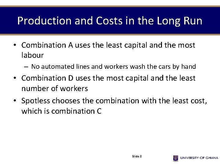
Production and Costs in the Long Run • Combination A uses the least capital and the most labour – No automated lines and workers wash the cars by hand • Combination D uses the most capital and the least number of workers • Spotless chooses the combination with the least cost, which is combination C Slide 8

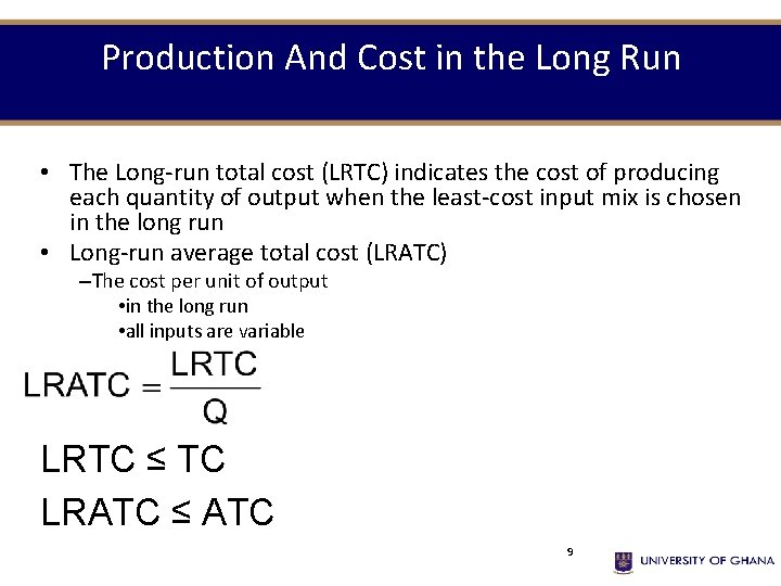
Production And Cost in the Long Run • The Long-run total cost (LRTC) indicates the cost of producing each quantity of output when the least-cost input mix is chosen in the long run • Long-run average total cost (LRATC) –The cost per unit of output • in the long run • all inputs are variable LRTC ≤ TC LRATC ≤ ATC 9

Topic One THE RELATIONSHIP BETWEEN LONG RUN COSTS AND SHORT RUN COSTS Slide 10

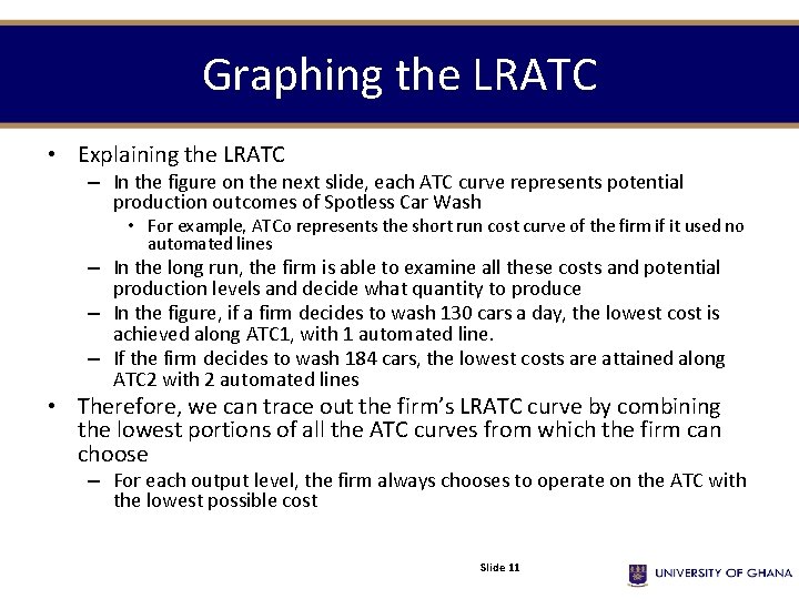
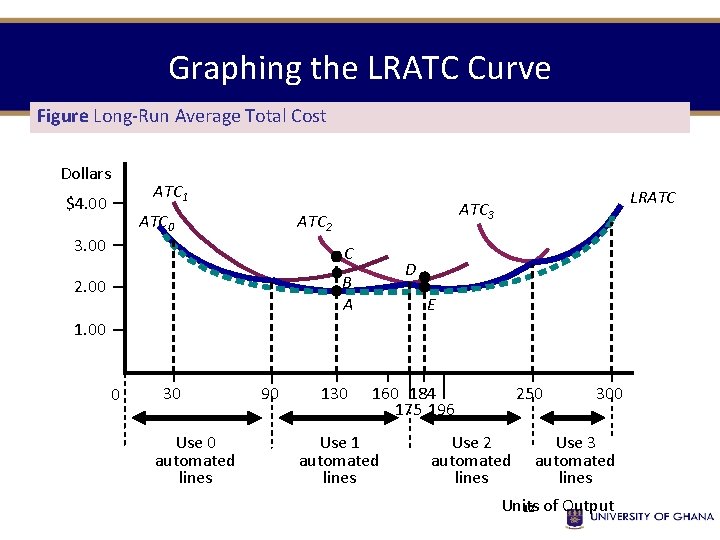
Graphing the LRATC • Explaining the LRATC – In the figure on the next slide, each ATC curve represents potential production outcomes of Spotless Car Wash • For example, ATCo represents the short run cost curve of the firm if it used no automated lines – In the long run, the firm is able to examine all these costs and potential production levels and decide what quantity to produce – In the figure, if a firm decides to wash 130 cars a day, the lowest cost is achieved along ATC 1, with 1 automated line. – If the firm decides to wash 184 cars, the lowest costs are attained along ATC 2 with 2 automated lines • Therefore, we can trace out the firm’s LRATC curve by combining the lowest portions of all the ATC curves from which the firm can choose – For each output level, the firm always chooses to operate on the ATC with the lowest possible cost Slide 11

Graphing the LRATC Curve Figure Long-Run Average Total Cost Dollars ATC 1 $4. 00 ATC 0 3. 00 ATC 2 C D B A 2. 00 LRATC 3 E 1. 00 0 30 Use 0 automated lines 90 130 160 184 175 196 Use 1 automated lines 250 Use 2 automated lines 300 Use 3 automated lines Units 12 of Output

Topic One EXPLAINING THE SHAPE OF THE LRATC CURVE Slide 13

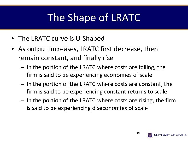
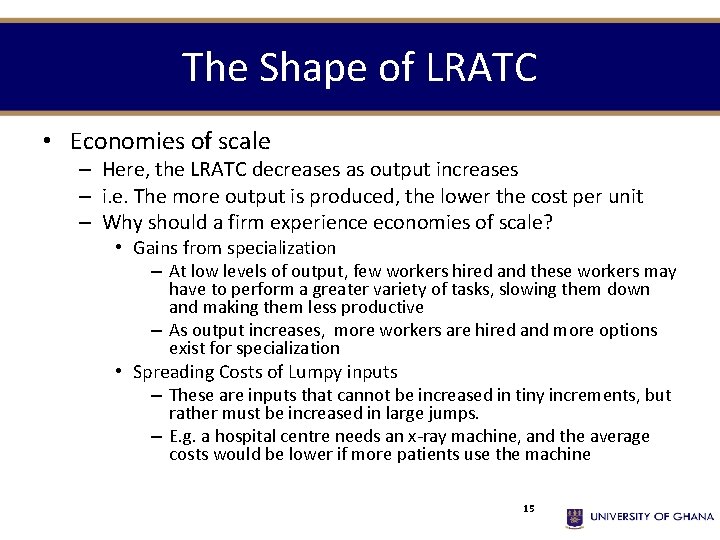
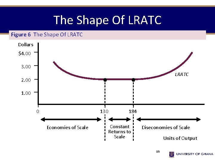
The Shape of LRATC • The LRATC curve is U-Shaped • As output increases, LRATC first decrease, then remain constant, and finally rise – In the portion of the LRATC where costs are falling, the firm is said to be experiencing economies of scale – In the portion of the LRATC where costs are constant, the firm is said to be experiencing constant returns to scale – In the portion of the LRATC where costs are rising, the firm is said to be experiencing diseconomies of scale 14

The Shape of LRATC • Economies of scale – Here, the LRATC decreases as output increases – i. e. The more output is produced, the lower the cost per unit – Why should a firm experience economies of scale? • Gains from specialization – At low levels of output, few workers hired and these workers may have to perform a greater variety of tasks, slowing them down and making them less productive – As output increases, more workers are hired and more options exist for specialization • Spreading Costs of Lumpy inputs – These are inputs that cannot be increased in tiny increments, but rather must be increased in large jumps. – E. g. a hospital centre needs an x-ray machine, and the average costs would be lower if more patients use the machine 15

The Shape of LRATC • Constant returns to scale • - LRATC is unchanged as output increases – LRATC curve is flat 16

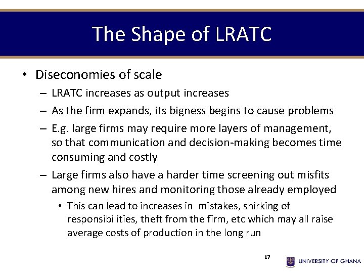
The Shape of LRATC • Diseconomies of scale – LRATC increases as output increases – As the firm expands, its bigness begins to cause problems – E. g. large firms may require more layers of management, so that communication and decision-making becomes time consuming and costly – Large firms also have a harder time screening out misfits among new hires and monitoring those already employed • This can lead to increases in mistakes, shirking of responsibilities, theft from the firm, etc which may all raise average costs of production in the long run 17

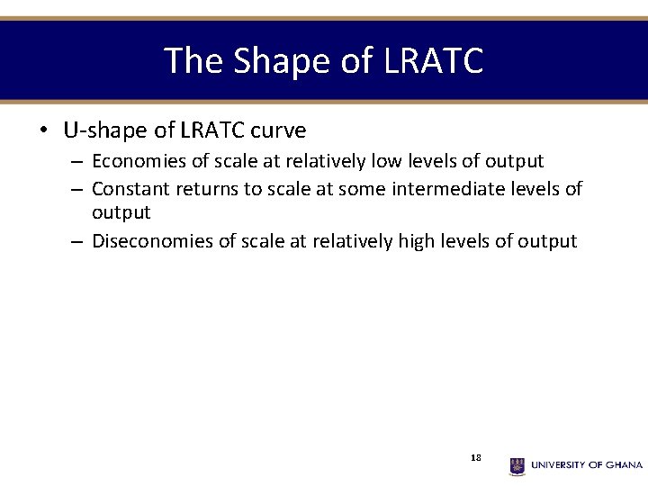
The Shape of LRATC • U-shape of LRATC curve – Economies of scale at relatively low levels of output – Constant returns to scale at some intermediate levels of output – Diseconomies of scale at relatively high levels of output 18

The Shape Of LRATC Figure 6 The Shape Of LRATC Dollars $4. 00 3. 00 LRATC 2. 00 130 0 Economies of Scale 184 Constant Returns to Scale Diseconomies of Scale Units of Output 19

References • Economics: Principles and Applications: Hall R. E. and Lieberman M. (2008), Thomson/ South Western (4 th Edition) Slide 20