ECO 365 Intermediate Microeconomics Lecture Notes Profit Maximization

ECO 365 – Intermediate Microeconomics Lecture Notes

Profit Maximization Profits (π) = TR – TC or π = ΣPi. Yi - Σ wj. Xj for i = 1 to n (outputs) and j = 1 to m (inputs). Types of Firms Proprietorship – single owner Partnership – two or more owners Corporation – firm is a separate legal entity Advantages and Disadvantages Factors of Production (Inputs) – 3 Types Variable inputs – varies with y. Fixed inputs – fixed even if y=0. Quasi-fixed inputs (if y=0 then x=0 but if y>0 then x is fixed).

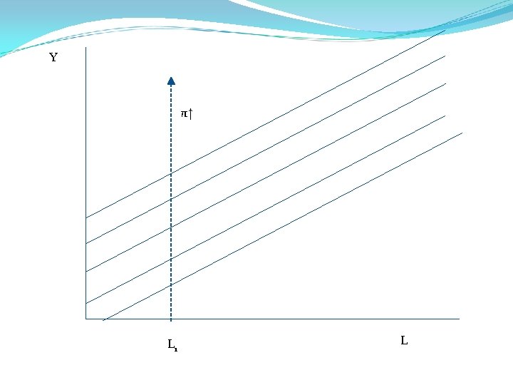
Short-run π maximization Assume only 1 output Y and two inputs L & K K is fixed => in short-run Firm problem is to choose L to maximize: Given that y = f(K, L) => choose L to max: How? MPL = w/p or p*MPL = w – what does this mean? Graphically Recall π = py – w. L – r. K, with K fixed or solve for y to get y = π/p + w. L/p + r. K/p Recall that p, w, r, and K are all fixed paramters, if we also hold π constant then we get a straight line in L, y space:

Y Slope = w/p Intercept = π /p + r. K/p L

The curve in the graph above is called an iso-profit curve. Why? Along a given iso-π then profit is fixed. If profit ↑ (↓) then the line shifts up (down). Thus, have a family of curves, all with same slope where profit increases as you move and decreases as you move down.

Y Isoprofit curve Y* L* L

Discuss the Graph above: Maximize profit by getting on highest iso-profit curve. Subject to constraint that must be on the production function. => tangency between the two or Slope of production function = slope of iso-profit or MPL = w/p – notice that this is the same condition as we already derived for profit maximization. What happens as P or w change? P ↑ or ↓ => what happens to L* and Y*? w ↑ or ↓ => what happens to L* and Y*? Show both graphically. Hint what happens to the slope of all isoprofit lines?

The Long-Run Maximize profit = pf(L, K) – w. L – r. K Both L and K are variable and hence a more complex problem. Recall that in the SR, profit max required MPL = w/p In LR is this still true? Also requires that MPK = r/p or P*MPK = r; P*MPL = w Both conditions must occur simultaneously Use these conditions to derive Factor Demand curves L* = f(p, w, r) and K* = f(p, w, r) Substitute these into production function to get optimal output Y = f(L*, K*)

Inverse factor demand curves w = f(L, K*, P) = P*MPL (L, K*) r = f(L*, K, P) = P*MPK (L*, K) or graphically – why downward sloping? w DL L

Returns to Scale What happens to profit with constant returns to scale? Inputs double => costs double => output doubles => profits double but => original output level was not profit max. What happens with increasing returns to scale? Problems If original profit = 0 => 2*0 = 0 => original profit may have been profit max. Eventually get decreasing returns to scale => what happens to profit? If firm size increases (Y increases) => under what conditions will P remain constant? Even if market competitive => if all firms increase Y => P will increase.

Revealed Profitability What is it? Suppose at time = t => with pt , wt, rt then the firm chooses Yt, Lt, and Kt. At a different time = s => with ps , ws, rs then the firm chooses Ys, Ls, and Ks. Must be true that: (1) pt Yt - wt Lt - rt Kt ≥ pt Ys - wt Ls - rt Ks - why? (2) ps Ys - ws Ls - rs Ks ≥ ps Yt - ws Lt - rs Kt - why? WAPM = Weak Axiom of Profit Maximization To be π maximization point the π from actual choices must be ≥ π from other possible choices at that time.

Implications of WAPM? Transform equation 2 to get: (3) -ps Yt + ws Lt + rs Kt ≥ -ps Ys + ws Ls + rs Ks Now add equations 3 and 1 together to get: (pt – ps)Yt – (wt – ws)Lt – (rt – rs)Kt ≥ (pt – ps)Ys - (wt – ws) Ls - (rt – rs)Ks or: (pt – ps)(Yt – Ys )– (wt – ws)(Lt - Ls) – (rt – rs)(Kt - Ks)≥ 0 Or (4) ΔpΔY – ΔwΔL – ΔrΔK ≥ 0 Suppose Δw = Δr = 0 => equation 4 implies that ΔpΔY ≥ 0 => if Δp > 0 then it must also be the case that ΔY > 0. What does this mean? Supply of the output is upward sloping

More implications of WAPM Suppose Δp = Δw = 0 => equation 4 implies that – ΔrΔK ≥ 0 or ΔrΔK ≤ 0 or if Δr ≥ 0 then it must be true that ΔK ≤ 0. What does this mean? Demand for Capital is downward sloping Do the same thing to show demand for labor is also downward sloping. Finally, note that profit maximization implies cost minimization (producing given Y with lowest costs). Why?