ECEN 667 Power System Stability Lecture 20 Voltage

ECEN 667 Power System Stability Lecture 20: Voltage Stability and Modal Analysis Prof. Tom Overbye Dept. of Electrical and Computer Engineering Texas A&M University overbye@tamu. edu Special Guest Lecture by TA Hanyue Li

Announcements • Read Chapter 8 • Homework 5 is due on Thursday Nov 14 1

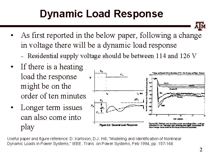
Dynamic Load Response • As first reported in the below paper, following a change in voltage there will be a dynamic load response – Residential supply voltage should be between 114 and 126 V • If there is a heating load the response might be on the order of ten minutes • Longer term issues can also come into play Useful paper and figure reference: D. Karlsson, D. J. Hill, “Modeling and Identification of Nonlinear Dynamic Loads in Power Systems, ” IEEE. Trans. on Power Systems, Feb 1994, pp. 157 -166 2

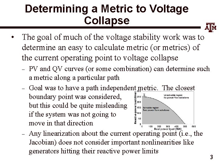
Determining a Metric to Voltage Collapse • The goal of much of the voltage stability work was to determine an easy to calculate metric (or metrics) of the current operating point to voltage collapse – – – PV and QV curves (or some combination) can determine such a metric along a particular path Goal was to have a path independent metric. The closest boundary point was considered, but this could be quite misleading if the system was not going to move in that direction Any linearization about the current operating point (i. e. , the Jacobian) does not consider important nonlinearities like generators hitting their reactive power limits 3

Assessing Voltage Margin Using PV and QV Curve Analysis • A common method for assessing the distance in parameter space to voltage instability (or an undesirable voltage profile) is to trace how the voltage magnitudes vary as the system parameters (such as the loads) are changed in a specified direction – If the direction involves changing the real power (P) this is known as a PV curve; if the change is with the reactive power (Q) then this is a QV curve • PV/QV curve analysis can be generalized to any parameter change, and can include the consideration of contingencies 4

PV and QV Analysis in Power. World • Requires setting up what is known in Power. World as an injection group – – An injection group specifies a set of objects, such as generators and loads, that can inject or absorb power Injection groups can be defined by selecting Case Information, Aggregation, Injection Groups • The PV and/or QV analysis then varies the injections in the injection group, tracing out the PV curve • This allows optional consideration of contingencies • The PV tool can be displayed by selecting Add-Ons, PV This has already been done in the Bus 2_PV case 5

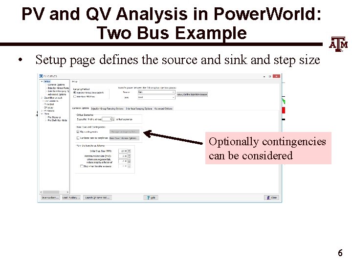
PV and QV Analysis in Power. World: Two Bus Example • Setup page defines the source and sink and step size Optionally contingencies can be considered 6

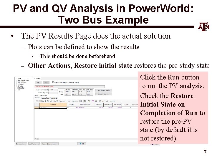
PV and QV Analysis in Power. World: Two Bus Example • The PV Results Page does the actual solution – Plots can be defined to show the results • – This should be done beforehand Other Actions, Restore initial state restores the pre-study state Click the Run button to run the PV analysis; Check the Restore Initial State on Completion of Run to restore the pre-PV state (by default it is not restored) 7

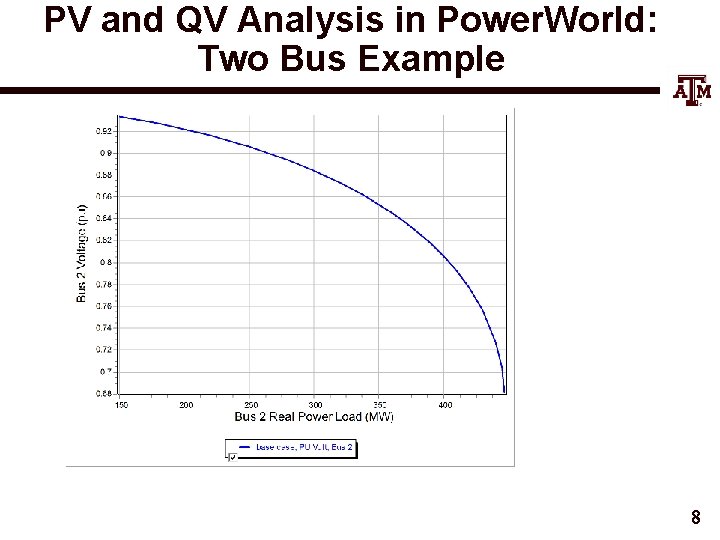
PV and QV Analysis in Power. World: Two Bus Example 8

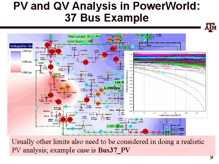
PV and QV Analysis in Power. World: 37 Bus Example Usually other limits also need to be considered in doing a realistic PV analysis; example case is Bus 37_PV 9

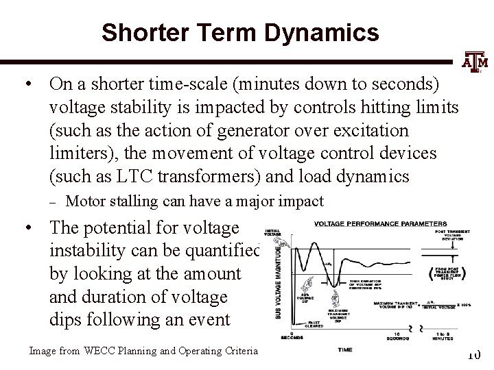
Shorter Term Dynamics • On a shorter time-scale (minutes down to seconds) voltage stability is impacted by controls hitting limits (such as the action of generator over excitation limiters), the movement of voltage control devices (such as LTC transformers) and load dynamics – Motor stalling can have a major impact • The potential for voltage instability can be quantified by looking at the amount and duration of voltage dips following an event Image from WECC Planning and Operating Criteria 10

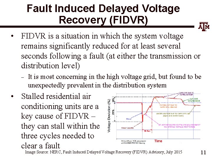
Fault Induced Delayed Voltage Recovery (FIDVR) • FIDVR is a situation in which the system voltage remains significantly reduced for at least several seconds following a fault (at either the transmission or distribution level) – It is most concerning in the high voltage grid, but found to be unexpectedly prevalent in the distribution system • Stalled residential air conditioning units are a key cause of FIDVR – they can stall within the three cycles needed to clear a fault Image Source: NERC, Fault Induced Delayed Voltage Recovery (FIDVR) Advisory, July 2015 11

Measurement-Based Modal Analysis • Measurement-based modal analysis determines the observed dynamic properties of a system – – Input can either be measurements from PMUs or transient stability results This is now more common, and has been implemented in Power. World Simulator 12

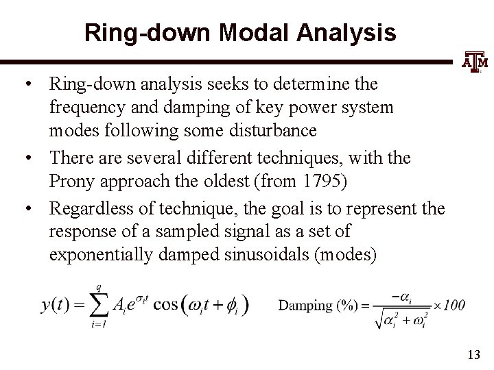
Ring-down Modal Analysis • Ring-down analysis seeks to determine the frequency and damping of key power system modes following some disturbance • There are several different techniques, with the Prony approach the oldest (from 1795) • Regardless of technique, the goal is to represent the response of a sampled signal as a set of exponentially damped sinusoidals (modes) 13

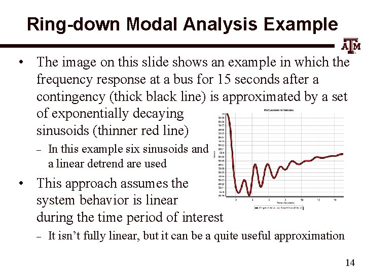
Ring-down Modal Analysis Example • The image on this slide shows an example in which the frequency response at a bus for 15 seconds after a contingency (thick black line) is approximated by a set of exponentially decaying sinusoids (thinner red line) – In this example six sinusoids and a linear detrend are used • This approach assumes the system behavior is linear during the time period of interest – It isn’t fully linear, but it can be a quite useful approximation 14

Modal Analysis in Power. World • Goal is to make modal analysis easy to use, and easy to visualize the results • Provided tool can be used with either transient stability results or actual system signals (e. g. , from PMUs) • Two ways to access in Power. World (with a quicker third way coming soon!) – – On the Transient Stability Analysis form left menu, Modal Analysis (right below SMIB Eigenvalues) By right-clicking on a transient stability or plot case information display, and selecting Modal Analysis Selected Columns or Modal Analysis All Columns 15

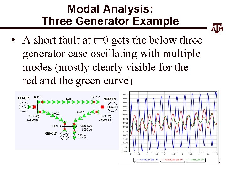
Modal Analysis: Three Generator Example • A short fault at t=0 gets the below three generator case oscillating with multiple modes (mostly clearly visible for the red and the green curve) 16

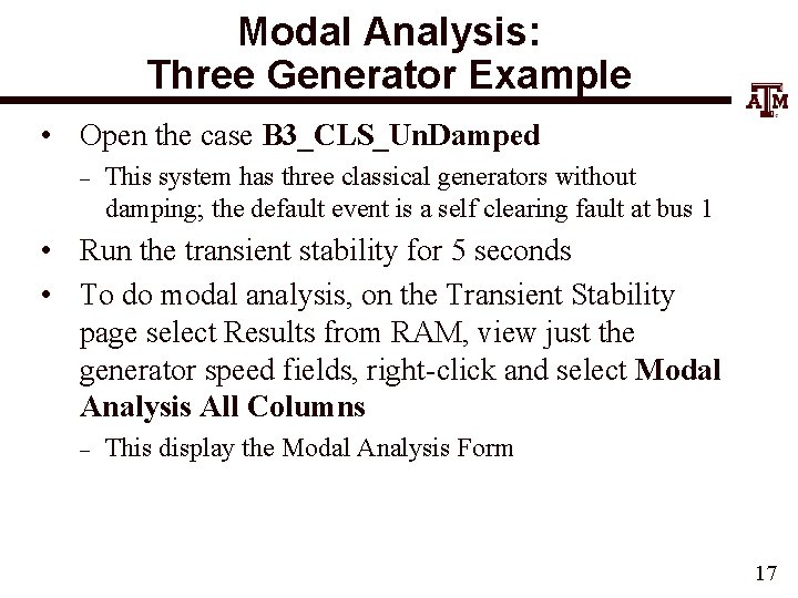
Modal Analysis: Three Generator Example • Open the case B 3_CLS_Un. Damped – This system has three classical generators without damping; the default event is a self clearing fault at bus 1 • Run the transient stability for 5 seconds • To do modal analysis, on the Transient Stability page select Results from RAM, view just the generator speed fields, right-click and select Modal Analysis All Columns – This display the Modal Analysis Form 17

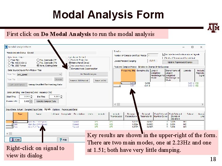
Modal Analysis Form First click on Do Modal Analysis to run the modal analysis Right-click on signal to view its dialog Key results are shown in the upper-right of the form. There are two main modes, one at 2. 23 Hz and one at 1. 51; both have very little damping. 18

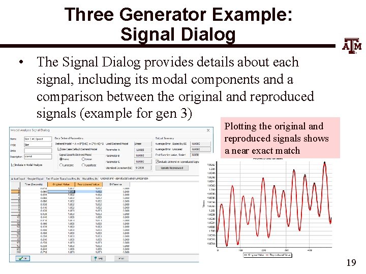
Three Generator Example: Signal Dialog • The Signal Dialog provides details about each signal, including its modal components and a comparison between the original and reproduced signals (example for gen 3) Plotting the original and reproduced signals shows a near exact match 19

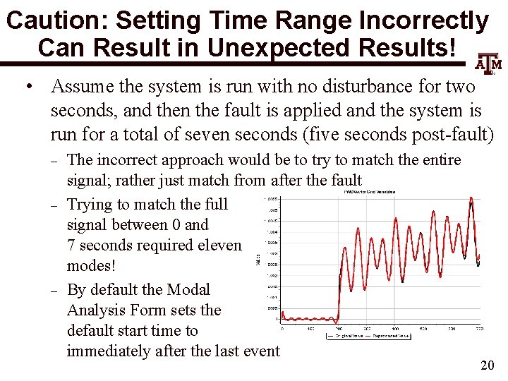
Caution: Setting Time Range Incorrectly Can Result in Unexpected Results! • Assume the system is run with no disturbance for two seconds, and then the fault is applied and the system is run for a total of seven seconds (five seconds post-fault) – – – The incorrect approach would be to try to match the entire signal; rather just match from after the fault Trying to match the full signal between 0 and 7 seconds required eleven modes! By default the Modal Analysis Form sets the default start time to immediately after the last event 20

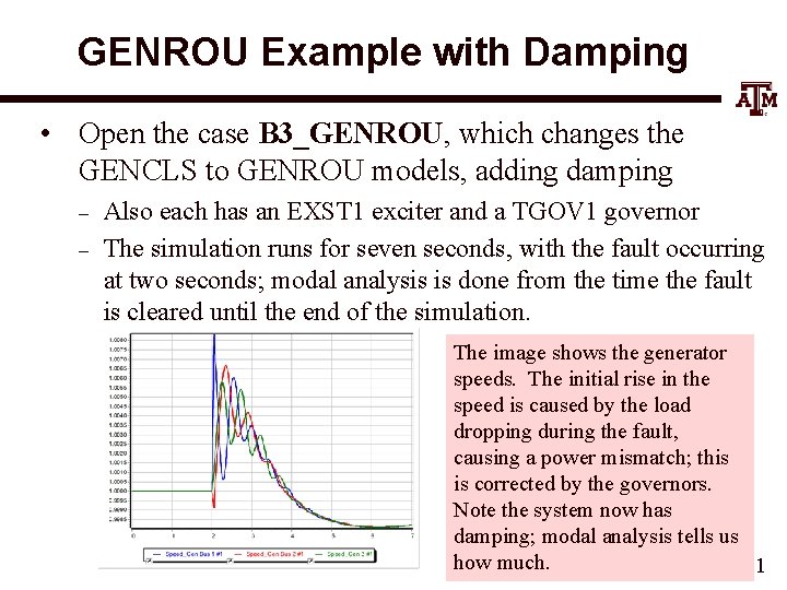
GENROU Example with Damping • Open the case B 3_GENROU, which changes the GENCLS to GENROU models, adding damping – – Also each has an EXST 1 exciter and a TGOV 1 governor The simulation runs for seven seconds, with the fault occurring at two seconds; modal analysis is done from the time the fault is cleared until the end of the simulation. The image shows the generator speeds. The initial rise in the speed is caused by the load dropping during the fault, causing a power mismatch; this is corrected by the governors. Note the system now has damping; modal analysis tells us how much. 21

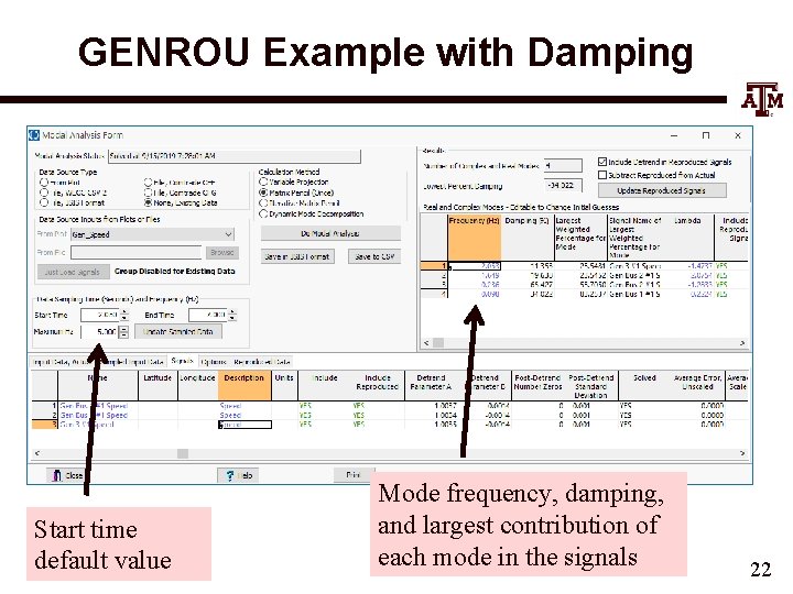
GENROU Example with Damping Start time default value Mode frequency, damping, and largest contribution of each mode in the signals 22

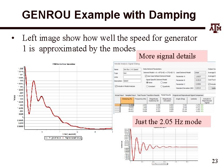
GENROU Example with Damping • Left image show well the speed for generator 1 is approximated by the modes More signal details Just the 2. 05 Hz mode 23

Signal-Based Modal Analysis • Idea of all techniques is to approximate a signal, yorg(t), by the sum of other, simpler signals (basis functions) – – Basis functions are usually exponentials, with linear and quadratic functions used to detrend the signal Properties of the original signal can be quantified from basis function properties • – Examples are frequency and damping Signal is considered over time with t=0 as the start • Approaches sample the original signal yorg(t) 24

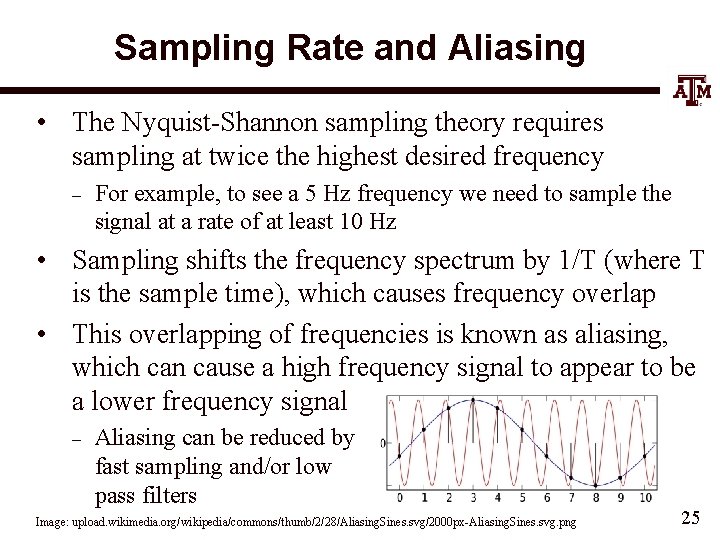
Sampling Rate and Aliasing • The Nyquist-Shannon sampling theory requires sampling at twice the highest desired frequency – For example, to see a 5 Hz frequency we need to sample the signal at a rate of at least 10 Hz • Sampling shifts the frequency spectrum by 1/T (where T is the sample time), which causes frequency overlap • This overlapping of frequencies is known as aliasing, which can cause a high frequency signal to appear to be a lower frequency signal – Aliasing can be reduced by fast sampling and/or low pass filters Image: upload. wikimedia. org/wikipedia/commons/thumb/2/28/Aliasing. Sines. svg/2000 px-Aliasing. Sines. svg. png 25

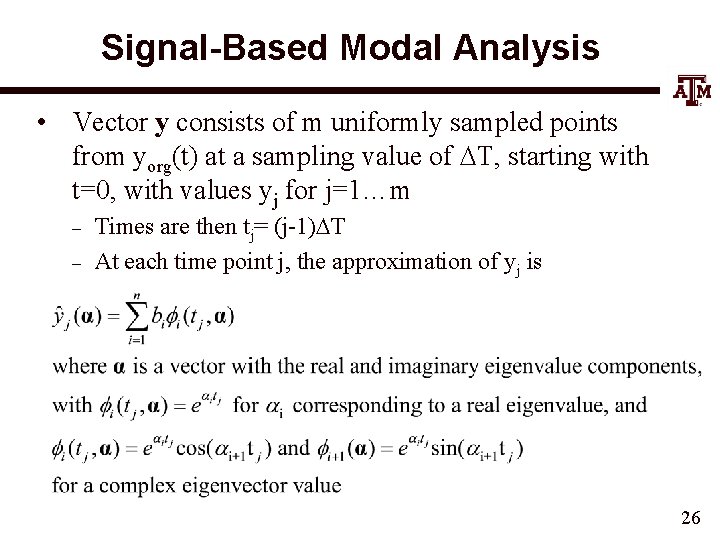
Signal-Based Modal Analysis • Vector y consists of m uniformly sampled points from yorg(t) at a sampling value of DT, starting with t=0, with values yj for j=1…m – – Times are then tj= (j-1)DT At each time point j, the approximation of yj is 26

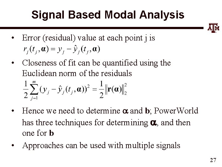
Signal Based Modal Analysis • Error (residual) value at each point j is • Closeness of fit can be quantified using the Euclidean norm of the residuals • Hence we need to determine a and b; Power. World has three techniques for determining a, and then one for b • Approaches can be used with multiple signals 27

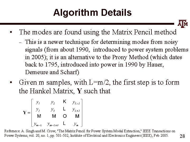
Algorithm Details • The modes are found using the Matrix Pencil method – This is a newer technique for determining modes from noisy signals (from about 1990, introduced to power system problems in 2005); it is an alternative to the Prony Method (which dates back to 1795, introduced into power in 1990 by Hauer, Demeure and Scharf) • Given m samples, with L=m/2, the first step is to form the Hankel Matrix, Y such that Refernece: A. Singh and M. Crow, "The Matrix Pencil for Power System Modal Extraction, " IEEE Transactions on Power Systems, vol. 20, no. 1, pp. 501 -502, Institute of Electrical and Electronics Engineers (IEEE), Feb 2005. 28

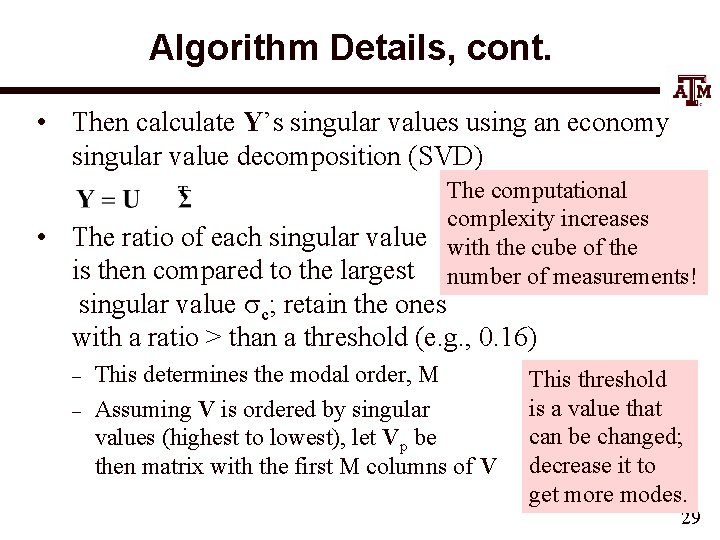
Algorithm Details, cont. • Then calculate Y’s singular values using an economy singular value decomposition (SVD) • The computational complexity increases The ratio of each singular value with the cube of the is then compared to the largest number of measurements! singular value sc; retain the ones with a ratio > than a threshold (e. g. , 0. 16) – – This determines the modal order, M Assuming V is ordered by singular values (highest to lowest), let Vp be then matrix with the first M columns of V This threshold is a value that can be changed; decrease it to get more modes. 29

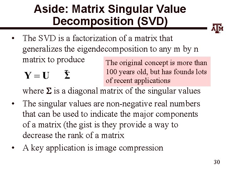
Aside: Matrix Singular Value Decomposition (SVD) • The SVD is a factorization of a matrix that generalizes the eigendecomposition to any m by n matrix to produce The original concept is more than 100 years old, but has founds lots of recent applications where S is a diagonal matrix of the singular values • The singular values are non-negative real numbers that can be used to indicate the major components of a matrix (the gist is they provide a way to decrease the rank of a matrix • A key application is image compression 30

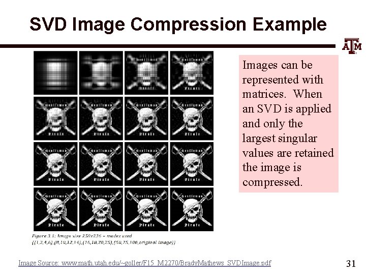
SVD Image Compression Example Images can be represented with matrices. When an SVD is applied and only the largest singular values are retained the image is compressed. Image Source: www. math. utah. edu/~goller/F 15_M 2270/Brady. Mathews_SVDImage. pdf 31

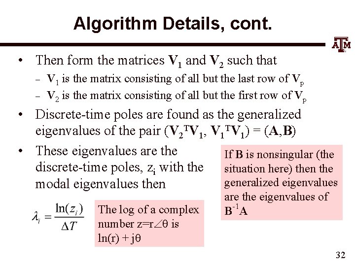
Algorithm Details, cont. • Then form the matrices V 1 and V 2 such that – – V 1 is the matrix consisting of all but the last row of Vp V 2 is the matrix consisting of all but the first row of Vp • Discrete-time poles are found as the generalized eigenvalues of the pair (V 2 TV 1, V 1 TV 1) = (A, B) • These eigenvalues are the If B is nonsingular (the discrete-time poles, zi with the situation here) then the generalized eigenvalues modal eigenvalues then The log of a complex number z=r is ln(r) + j are the eigenvalues of B-1 A 32

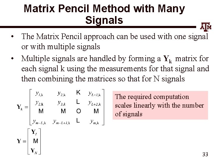
Matrix Pencil Method with Many Signals • The Matrix Pencil approach can be used with one signal or with multiple signals • Multiple signals are handled by forming a Yk matrix for each signal k using the measurements for that signal and then combining the matrices so that for N signals The required computation scales linearly with the number of signals 33

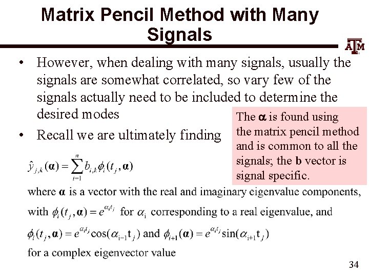
Matrix Pencil Method with Many Signals • However, when dealing with many signals, usually the signals are somewhat correlated, so vary few of the signals actually need to be included to determine the desired modes The a is found using • Recall we are ultimately finding the matrix pencil method and is common to all the signals; the b vector is signal specific. 34

Iterative Matrix Pencil Method • When there a large number of signals the iterative matrix pencil method works by – – – Selecting an initial signal to calculate the a vector Quickly calculating the b vectors for all the signals, and getting a cost function for how closely the reconstructed signals match their sampled values Selecting a signal that has a high cost function, and repeating the above adding this signal to the algorithm to get an updated a 35