ECEN 460 Power System Operation and Control Lecture

ECEN 460 Power System Operation and Control Lecture 15: Economic Dispatch Adam Birchfield Dept. of Electrical and Computer Engineering Texas A&M University abirchfield@tamu. edu Material gratefully adapted with permission from slides by Prof. Tom Overbye.

1 Announcements • Finish reading Chapter 6 • Homework 5 is 6. 38 (use Z = 0. 02+j 0. 08), 6. 39 (use Z = 0. 02+j 0. 08), 6. 44, 6. 48, 6. 52, 6. 53; – Due on Thursday Oct 25 • Lab 6 this week 10/19, 10/22, 10/23

2 Generation Dispatch • • Since the load is variable and there must be enough generation to meet the load, almost always there is more generation capacity available than load Optimally determining which generators to use can be a complicated task due to many different constraints – – – • For generators with low or no cost fuel (e. g. , wind and solar PV) it is “use it or lose it” For others like hydro there may be limited energy for the year Some fossil has shut down and start times of many hours Economic dispatch looks at the best way to instantaneously dispatch the generation

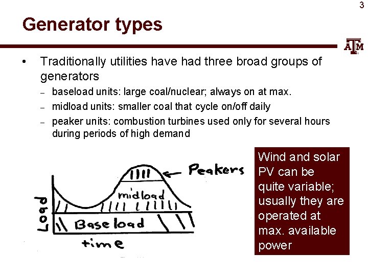
3 Generator types • Traditionally utilities have had three broad groups of generators – – – baseload units: large coal/nuclear; always on at max. midload units: smaller coal that cycle on/off daily peaker units: combustion turbines used only for several hours during periods of high demand Wind and solar PV can be quite variable; usually they are operated at max. available power

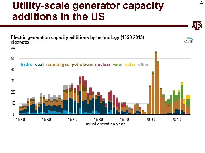
Utility-scale generator capacity additions in the US 4

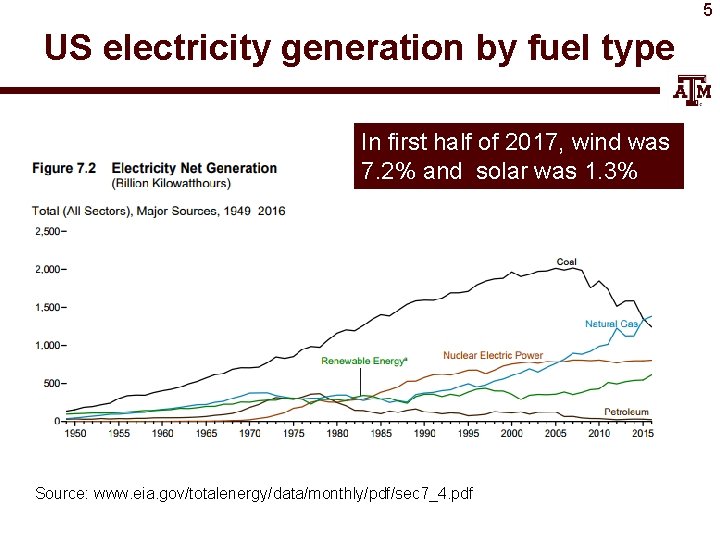
5 US electricity generation by fuel type In first half of 2017, wind was 7. 2% and solar was 1. 3% Source: www. eia. gov/totalenergy/data/monthly/pdf/sec 7_4. pdf

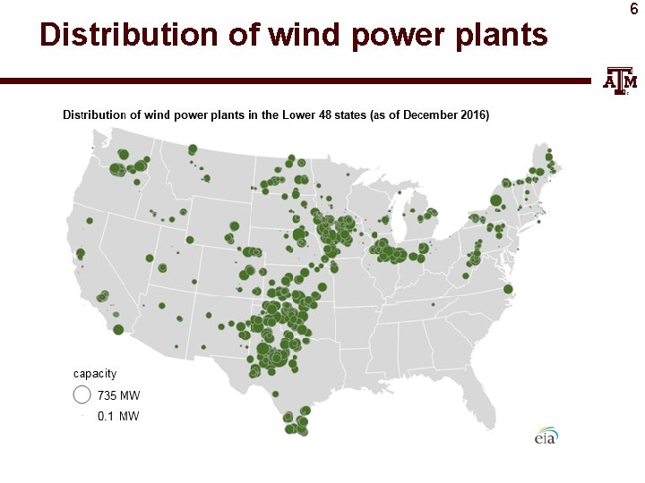
Distribution of wind power plants 6

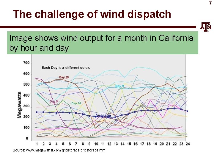
7 The challenge of wind dispatch Image shows wind output for a month in California by hour and day Source: www. megawattsf. com/gridstorage. htm

8 Thermal versus hydro generation • • The two main types of generating units are thermal and hydro, with wind rapidly growing For hydro the fuel (water) is free but there may be many constraints on operation – – – • • fixed amounts of water available reservoir levels must be managed and coordinated downstream flow rates for fish and navigation Hydro optimization is typically longer term (many months or years) In 460 we will concentrate on thermal units and some wind, looking at short-term optimization

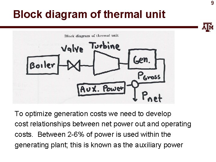
9 Block diagram of thermal unit To optimize generation costs we need to develop cost relationships between net power out and operating costs. Between 2 -6% of power is used within the generating plant; this is known as the auxiliary power

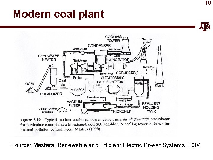
10 Modern coal plant Source: Masters, Renewable and Efficient Electric Power Systems, 2004

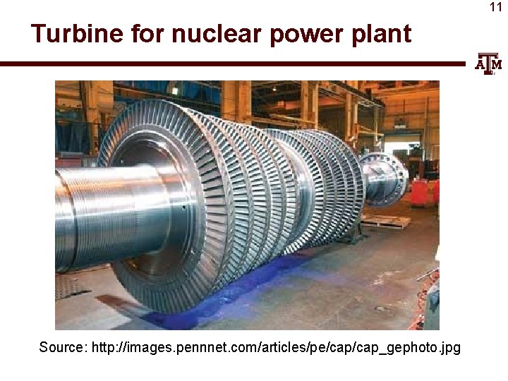
11 Turbine for nuclear power plant Source: http: //images. pennnet. com/articles/pe/cap_gephoto. jpg

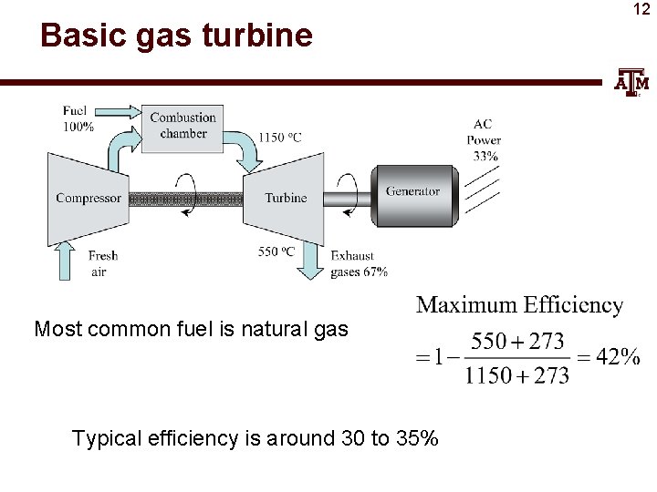
Basic gas turbine Most common fuel is natural gas Typical efficiency is around 30 to 35% 12

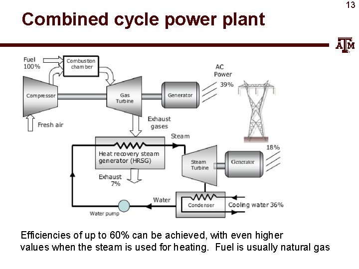
Combined cycle power plant Efficiencies of up to 60% can be achieved, with even higher values when the steam is used for heating. Fuel is usually natural gas 13

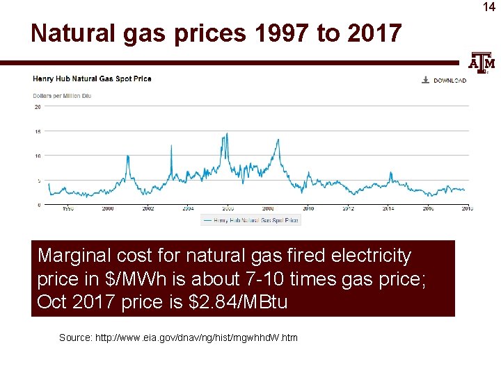
14 Natural gas prices 1997 to 2017 Marginal cost for natural gas fired electricity price in $/MWh is about 7 -10 times gas price; Oct 2017 price is $2. 84/MBtu Source: http: //www. eia. gov/dnav/ng/hist/rngwhhd. W. htm

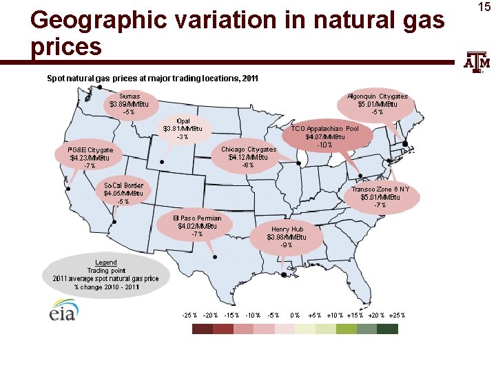
Geographic variation in natural gas prices 15

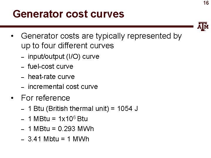
16 Generator cost curves • Generator costs are typically represented by up to four different curves – – input/output (I/O) curve fuel-cost curve heat-rate curve incremental cost curve • For reference – – 1 Btu (British thermal unit) = 1054 J 1 MBtu = 1 x 106 Btu 1 MBtu = 0. 293 MWh 3. 41 Mbtu = 1 MWh

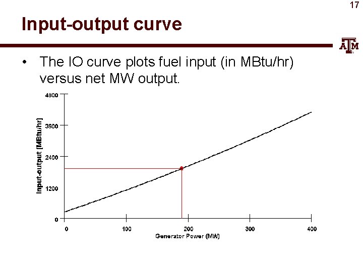
17 Input-output curve • The IO curve plots fuel input (in MBtu/hr) versus net MW output.

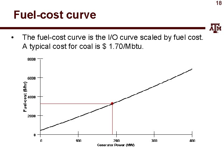
18 Fuel-cost curve • The fuel-cost curve is the I/O curve scaled by fuel cost. A typical cost for coal is $ 1. 70/Mbtu.

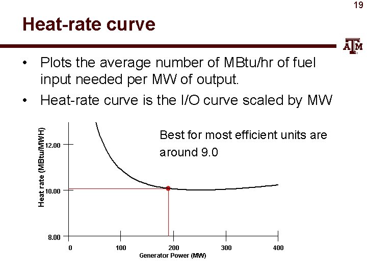
19 Heat-rate curve • Plots the average number of MBtu/hr of fuel input needed per MW of output. • Heat-rate curve is the I/O curve scaled by MW Best for most efficient units are around 9. 0

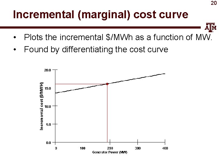
20 Incremental (marginal) cost curve • Plots the incremental $/MWh as a function of MW. • Found by differentiating the cost curve

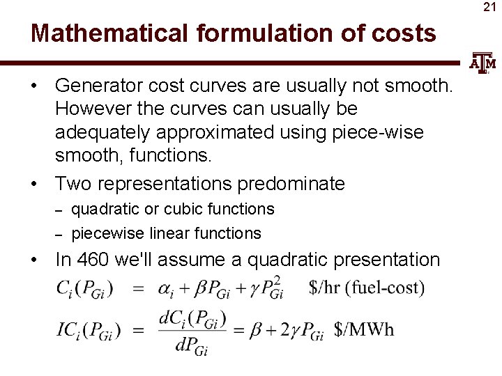
21 Mathematical formulation of costs • Generator cost curves are usually not smooth. However the curves can usually be adequately approximated using piece-wise smooth, functions. • Two representations predominate – – quadratic or cubic functions piecewise linear functions • In 460 we'll assume a quadratic presentation

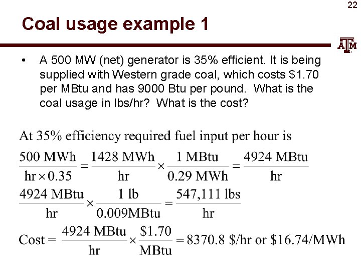
22 Coal usage example 1 • A 500 MW (net) generator is 35% efficient. It is being supplied with Western grade coal, which costs $1. 70 per MBtu and has 9000 Btu per pound. What is the coal usage in lbs/hr? What is the cost?

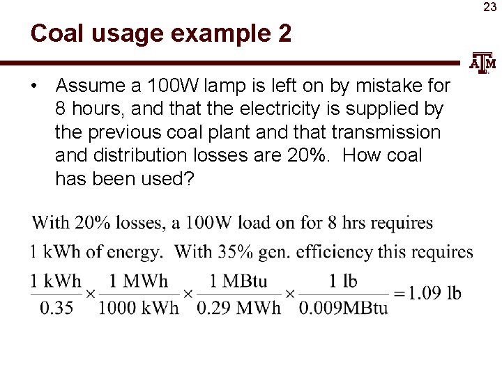
23 Coal usage example 2 • Assume a 100 W lamp is left on by mistake for 8 hours, and that the electricity is supplied by the previous coal plant and that transmission and distribution losses are 20%. How coal has been used?

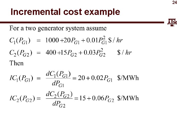
24 Incremental cost example

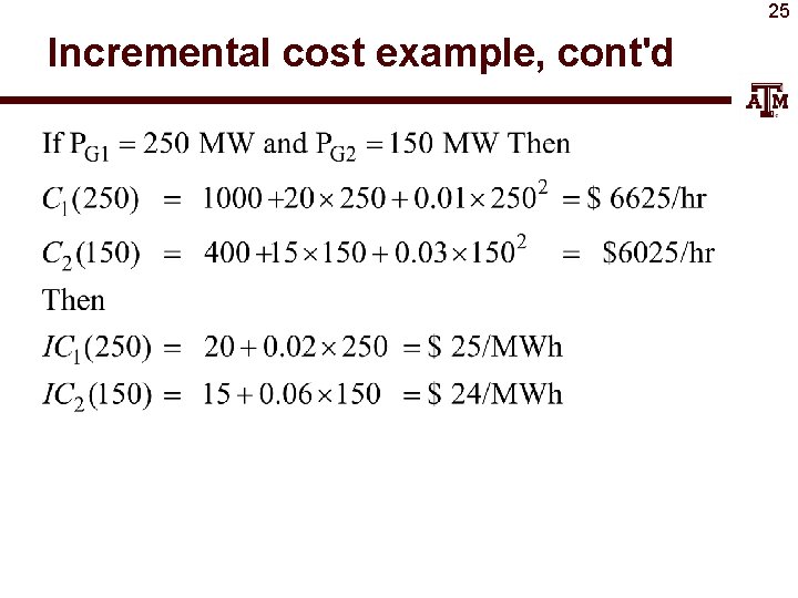
25 Incremental cost example, cont'd

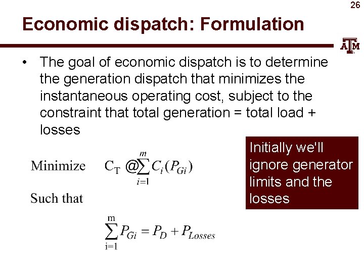
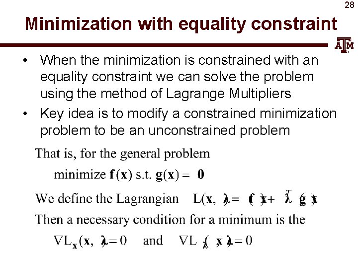
26 Economic dispatch: Formulation • The goal of economic dispatch is to determine the generation dispatch that minimizes the instantaneous operating cost, subject to the constraint that total generation = total load + losses Initially we'll ignore generator limits and the losses

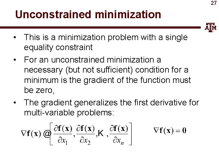
27 Unconstrained minimization • This is a minimization problem with a single equality constraint • For an unconstrained minimization a necessary (but not sufficient) condition for a minimum is the gradient of the function must be zero, • The gradient generalizes the first derivative for multi-variable problems:

28 Minimization with equality constraint • When the minimization is constrained with an equality constraint we can solve the problem using the method of Lagrange Multipliers • Key idea is to modify a constrained minimization problem to be an unconstrained problem

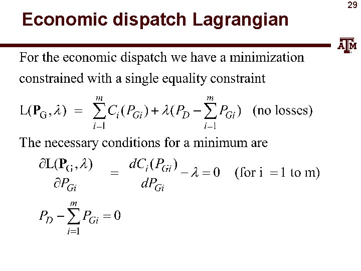
Economic dispatch Lagrangian 29

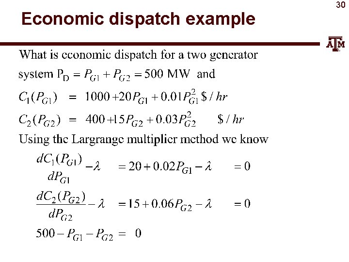
Economic dispatch example 30

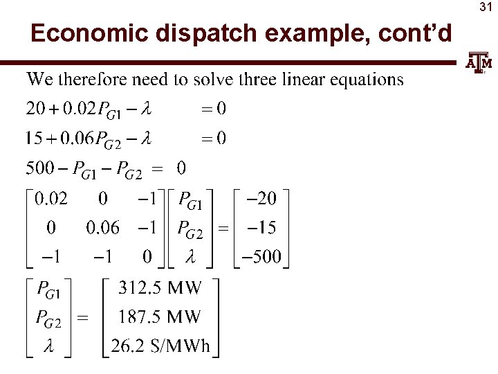
31 Economic dispatch example, cont’d

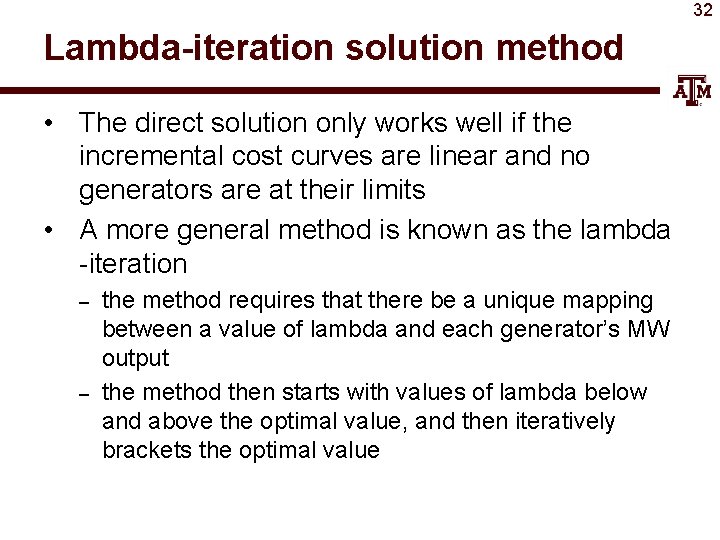
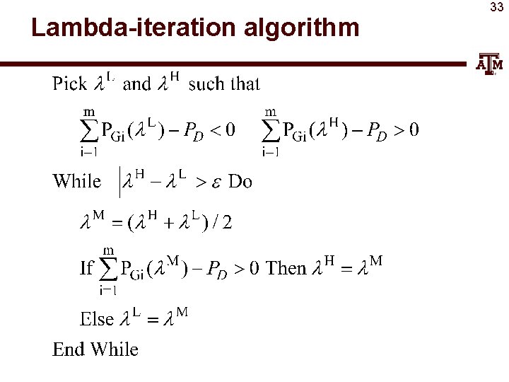
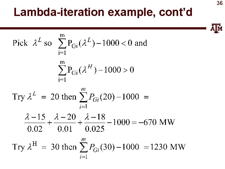
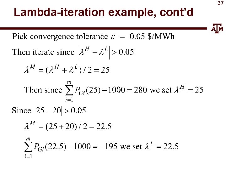
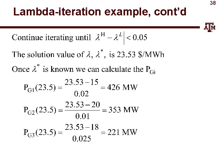
32 Lambda-iteration solution method • The direct solution only works well if the incremental cost curves are linear and no generators are at their limits • A more general method is known as the lambda -iteration – – the method requires that there be a unique mapping between a value of lambda and each generator’s MW output the method then starts with values of lambda below and above the optimal value, and then iteratively brackets the optimal value

Lambda-iteration algorithm 33

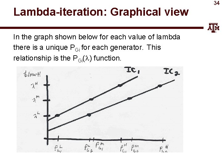
Lambda-iteration: Graphical view In the graph shown below for each value of lambda there is a unique PGi for each generator. This relationship is the PGi( ) function. 34

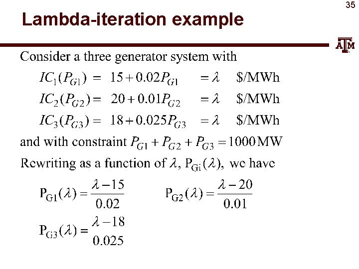
Lambda-iteration example 35

Lambda-iteration example, cont’d 36

Lambda-iteration example, cont’d 37

Lambda-iteration example, cont’d 38

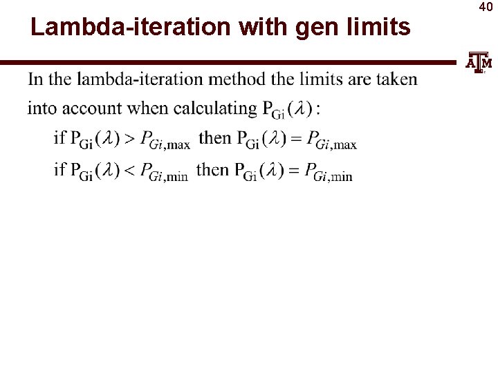
39 Generator MW limits • Generators have limits on the minimum and maximum amount of power they can produce • Often times the minimum limit is not zero. This represents a limit on the generator’s operation with the desired fuel type • Because of varying system economics usually many generators in a system are operated at their maximum MW limits.

Lambda-iteration with gen limits 40

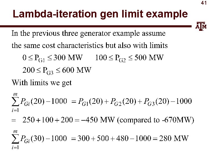
41 Lambda-iteration gen limit example

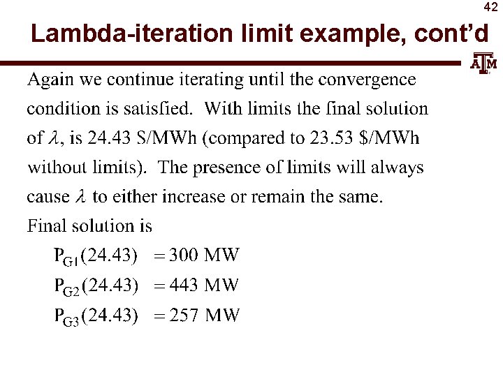
42 Lambda-iteration limit example, cont’d

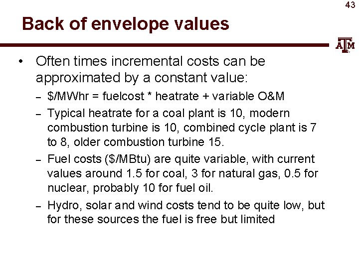
43 Back of envelope values • Often times incremental costs can be approximated by a constant value: – – $/MWhr = fuelcost * heatrate + variable O&M Typical heatrate for a coal plant is 10, modern combustion turbine is 10, combined cycle plant is 7 to 8, older combustion turbine 15. Fuel costs ($/MBtu) are quite variable, with current values around 1. 5 for coal, 3 for natural gas, 0. 5 for nuclear, probably 10 for fuel oil. Hydro, solar and wind costs tend to be quite low, but for these sources the fuel is free but limited

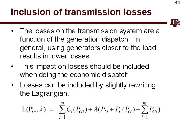
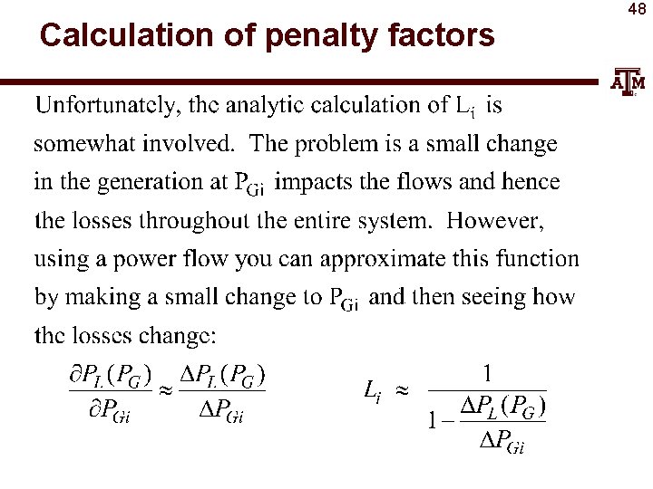
44 Inclusion of transmission losses • The losses on the transmission system are a function of the generation dispatch. In general, using generators closer to the load results in lower losses • This impact on losses should be included when doing the economic dispatch • Losses can be included by slightly rewriting the Lagrangian:

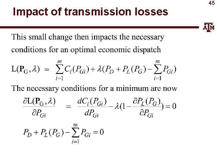
Impact of transmission losses 45

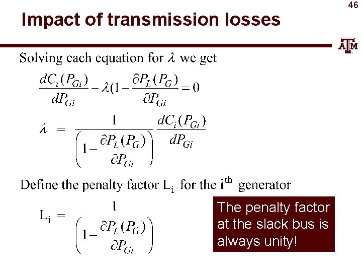
Impact of transmission losses The penalty factor at the slack bus is always unity! 46

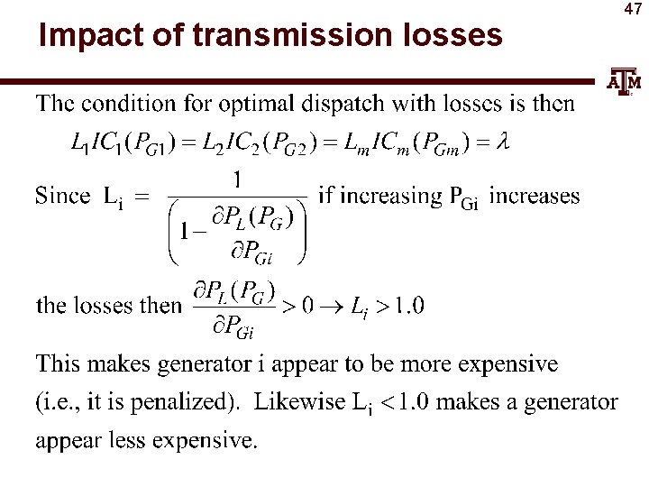
Impact of transmission losses 47

Calculation of penalty factors 48

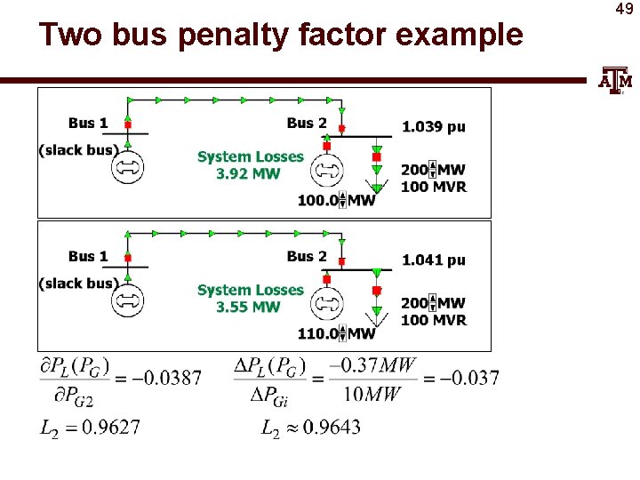
Two bus penalty factor example 49

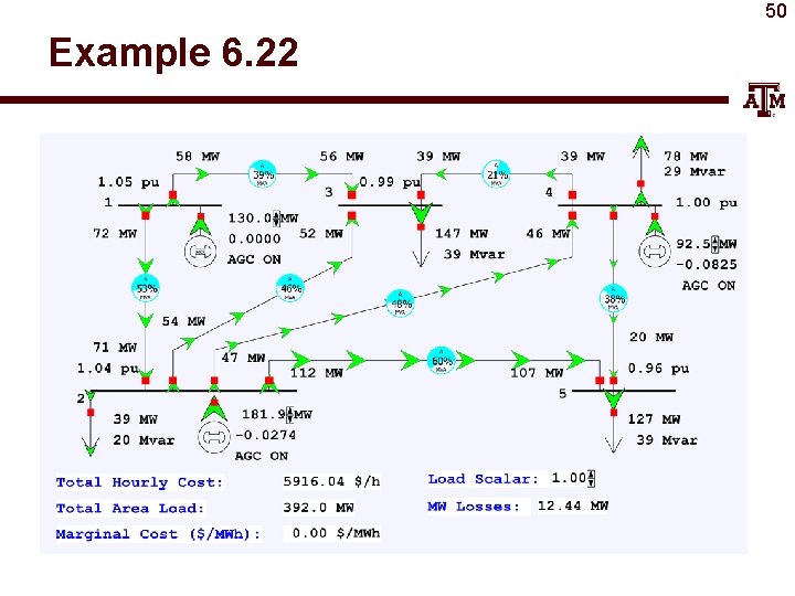
50 Example 6. 22

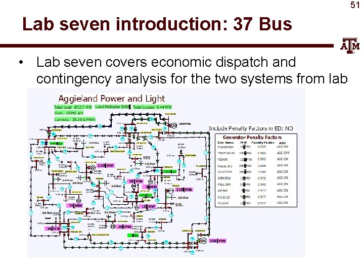
51 Lab seven introduction: 37 Bus • Lab seven covers economic dispatch and contingency analysis for the two systems from lab six

52 Lab seven introduction: 37 Bus • Lab considers the system economic dispatch under varying load conditions, using a uniform load scalar • In first part of lab you’ll observe how values change without consideration of losses • Second part is a repeat considering the impact of marginal losses • Third part looks at contingency analysis, with the goal to fix voltage and flow violations • Last part looks at loss minimization

Contingency analysis and the reference case 53 • Contingency analysis works by first storing a reference case, then sequentially applying each contingency to the reference case, reloading the reference case between contingencies • In Power. World the reference case can be changed by either closing and reopening the contingency analysis form, or using an option on the form • This allows you to easily look at of individual contingency cases – Right click on the contingencies and select Contingency Records, Solve Selected Contingency

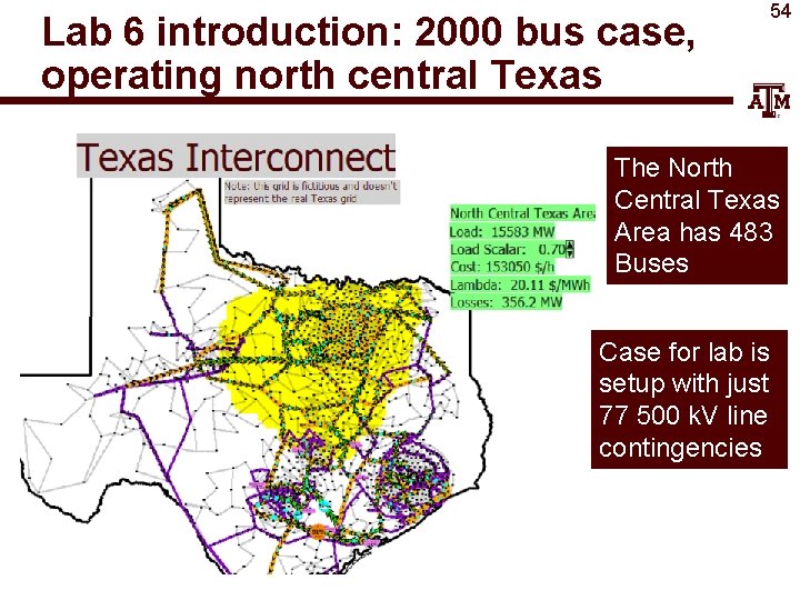
Lab 6 introduction: 2000 bus case, operating north central Texas 54 The North Central Texas Area has 483 Buses Case for lab is setup with just 77 500 k. V line contingencies

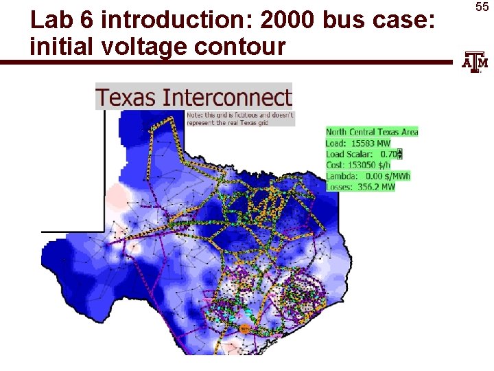
Lab 6 introduction: 2000 bus case: initial voltage contour 55