ECE 8527 to Machine Learning and Pattern Recognition

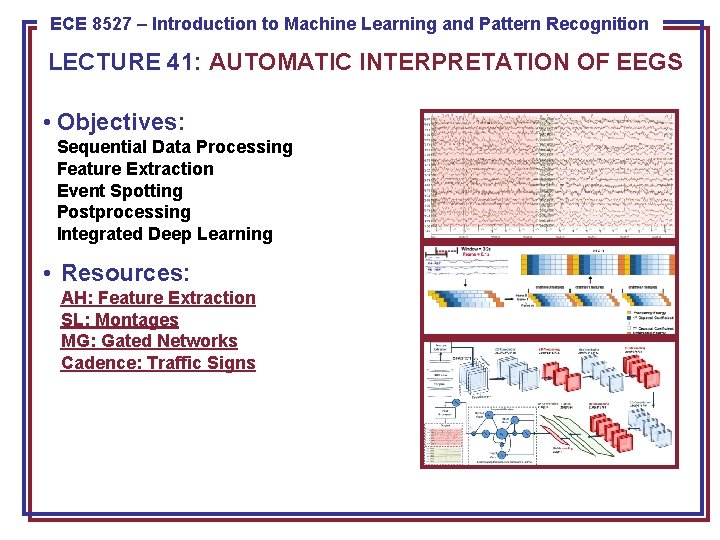
ECE 8527 to Machine Learning and Pattern Recognition 8443 – Introduction Pattern Recognition LECTURE 41: AUTOMATIC INTERPRETATION OF EEGS • Objectives: Sequential Data Processing Feature Extraction Event Spotting Postprocessing Integrated Deep Learning • Resources: AH: Feature Extraction SL: Montages MG: Gated Networks Cadence: Traffic Signs

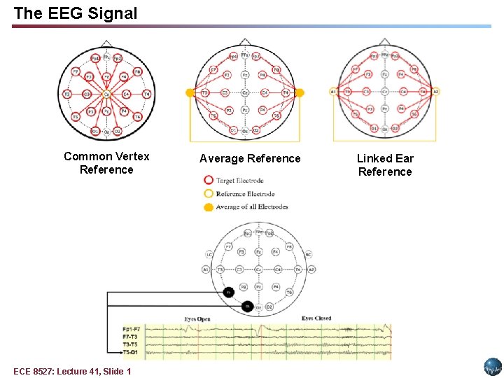
The EEG Signal Common Vertex Reference ECE 8527: Lecture 41, Slide 1 Average Reference Linked Ear Reference

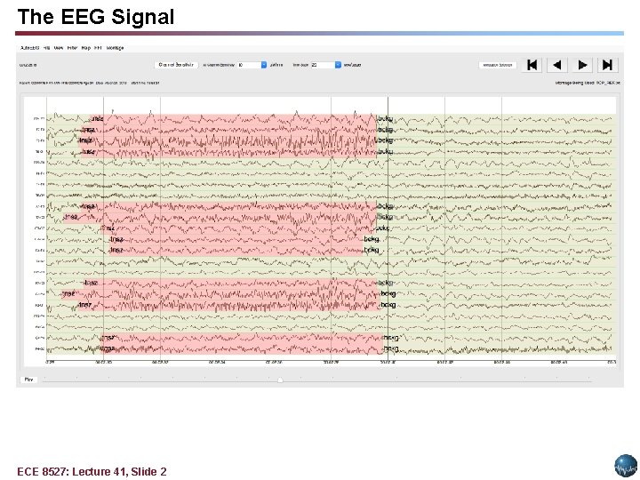
The EEG Signal ECE 8527: Lecture 41, Slide 2

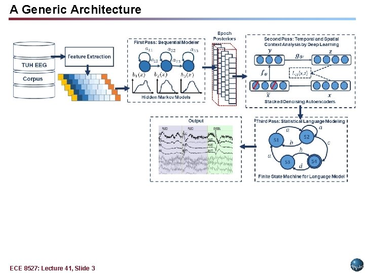
A Generic Architecture ECE 8527: Lecture 41, Slide 3

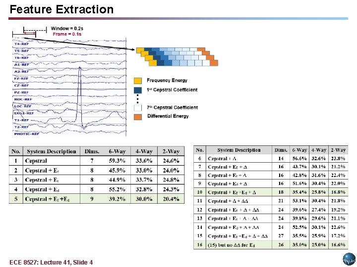
Feature Extraction ECE 8527: Lecture 41, Slide 4

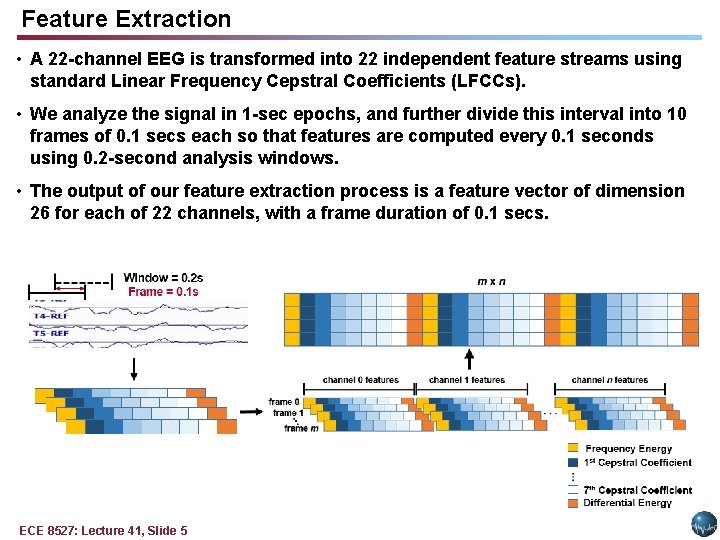
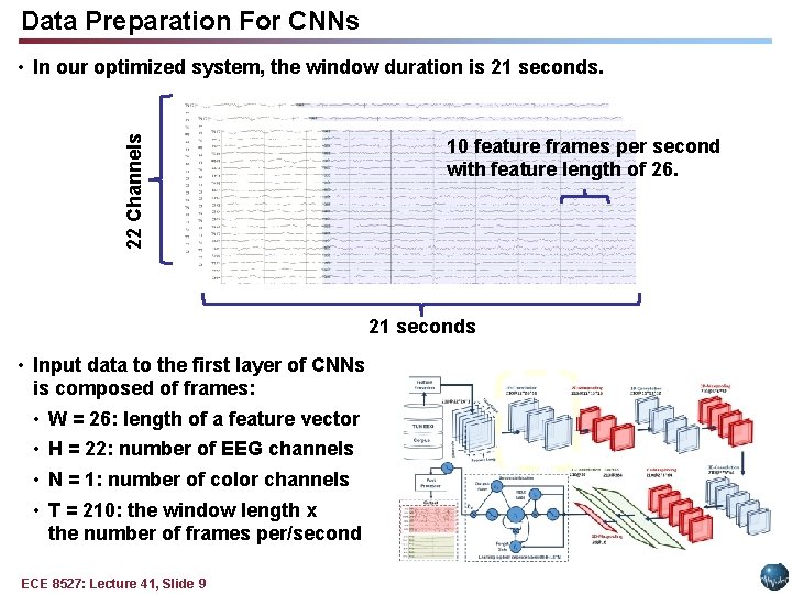
Feature Extraction • A 22 -channel EEG is transformed into 22 independent feature streams using standard Linear Frequency Cepstral Coefficients (LFCCs). • We analyze the signal in 1 -sec epochs, and further divide this interval into 10 frames of 0. 1 secs each so that features are computed every 0. 1 seconds using 0. 2 -second analysis windows. • The output of our feature extraction process is a feature vector of dimension 26 for each of 22 channels, with a frame duration of 0. 1 secs. ECE 8527: Lecture 41, Slide 5

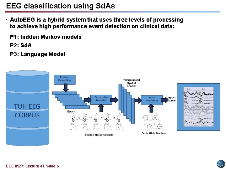
EEG classification using Sd. As • Auto. EEG is a hybrid system that uses three levels of processing to achieve high performance event detection on clinical data: P 1: hidden Markov models P 2: Sd. A P 3: Language Model ECE 8527: Lecture 41, Slide 6

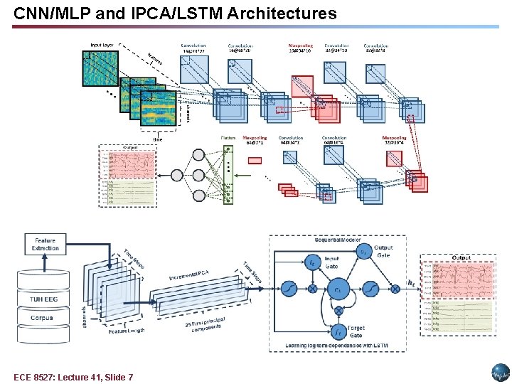
CNN/MLP and IPCA/LSTM Architectures ECE 8527: Lecture 41, Slide 7

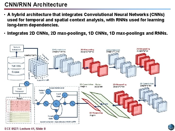
CNN/RNN Architecture • A hybrid architecture that integrates Convolutional Neural Networks (CNNs) used for temporal and spatial context analysis, with RNNs used for learning long-term dependencies. • Integrates 2 D CNNs, 2 D max-poolings, 1 D CNNs, 1 D max-poolings and RNNs. ECE 8527: Lecture 41, Slide 8

Data Preparation For CNNs 22 Channels • In our optimized system, the window duration is 21 seconds. 10 feature frames per second with feature length of 26. 21 seconds • Input data to the first layer of CNNs is composed of frames: • W = 26: length of a feature vector • H = 22: number of EEG channels • N = 1: number of color channels • T = 210: the window length x the number of frames per/second ECE 8527: Lecture 41, Slide 9

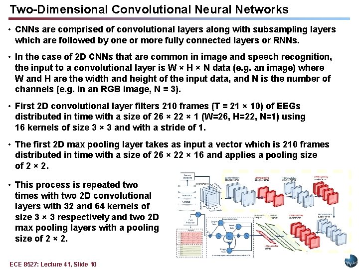
Two-Dimensional Convolutional Neural Networks • CNNs are comprised of convolutional layers along with subsampling layers which are followed by one or more fully connected layers or RNNs. • In the case of 2 D CNNs that are common in image and speech recognition, the input to a convolutional layer is W × H × N data (e. g. an image) where W and H are the width and height of the input data, and N is the number of channels (e. g. in an RGB image, N = 3). • First 2 D convolutional layer filters 210 frames (T = 21 × 10) of EEGs distributed in time with a size of 26 × 22 × 1 (W=26, H=22, N=1) using 16 kernels of size 3 × 3 and with a stride of 1. • The first 2 D max pooling layer takes as input a vector which is 210 frames distributed in time with a size of 26 × 22 × 16 and applies a pooling size of 2 × 2. • This process is repeated two times with two 2 D convolutional layers with 32 and 64 kernels of size 3 × 3 respectively and two 2 D max pooling layers with a pooling size of 2 × 2. ECE 8527: Lecture 41, Slide 10

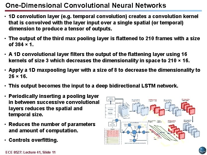
One-Dimensional Convolutional Neural Networks • 1 D convolution layer (e. g. temporal convolution) creates a convolution kernel that is convolved with the layer input over a single spatial (or temporal) dimension to produce a tensor of outputs. • The output of the third max pooling layer is flattened to 210 frames with a size of 384 × 1. • A 1 D convolutional layer filters the output of the flattening layer using 16 kernels of size 3 which decreases the dimensionality in space to 210 × 16. • Apply a 1 D maxpooling layer with a size of 8 to decrease the dimensionality to 26 × 16. • This output becomes the input to a deep bidirectional LSTM network. • Periodically inserting a pooling layer in between successive convolutional layers reduces the spatial and temporal size. • Reduces the number of parameters and amount of computation. • Controls overfitting. ECE 8527: Lecture 41, Slide 11

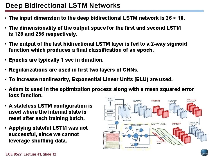
Deep Bidirectional LSTM Networks • The input dimension to the deep bidirectional LSTM network is 26 × 16. • The dimensionality of the output space for the first and second LSTM is 128 and 256 respectively. • The output of the last bidirectional LSTM layer is fed to a 2 -way sigmoid function which produces a final classification of an epoch. • Epochs are typically 1 sec in duration. • Regularizations are used in first two layers of CNNs. • To increase nonlinearity, Exponential Linear Units (ELU) are used. • Adam is used in the optimization process along with a mean squared error loss function. • A stateless LSTM configuration is used where the internal state is reset after each training batch. • Applying stateful LSTM was not successful, since we cannot leverage shuffling data. ECE 8527: Lecture 41, Slide 12

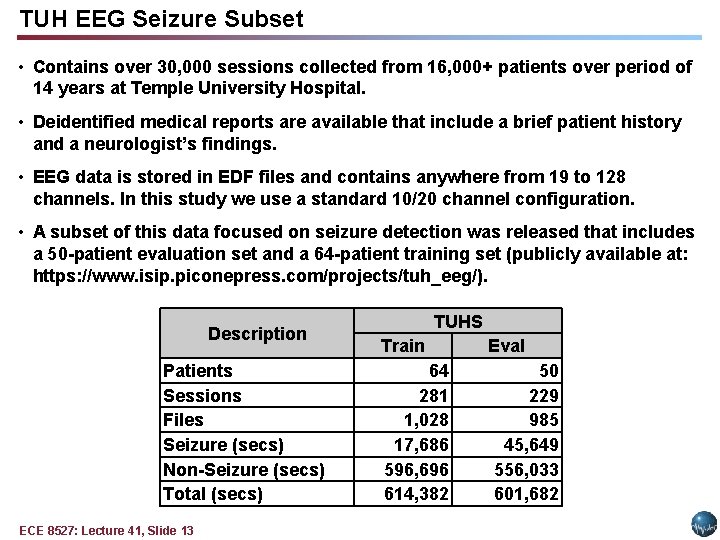
TUH EEG Seizure Subset • Contains over 30, 000 sessions collected from 16, 000+ patients over period of 14 years at Temple University Hospital. • Deidentified medical reports are available that include a brief patient history and a neurologist’s findings. • EEG data is stored in EDF files and contains anywhere from 19 to 128 channels. In this study we use a standard 10/20 channel configuration. • A subset of this data focused on seizure detection was released that includes a 50 -patient evaluation set and a 64 -patient training set (publicly available at: https: //www. isip. piconepress. com/projects/tuh_eeg/). Description Patients Sessions Files Seizure (secs) Non-Seizure (secs) Total (secs) ECE 8527: Lecture 41, Slide 13 TUHS Train 64 281 1, 028 17, 686 596, 696 614, 382 Eval 50 229 985 45, 649 556, 033 601, 682

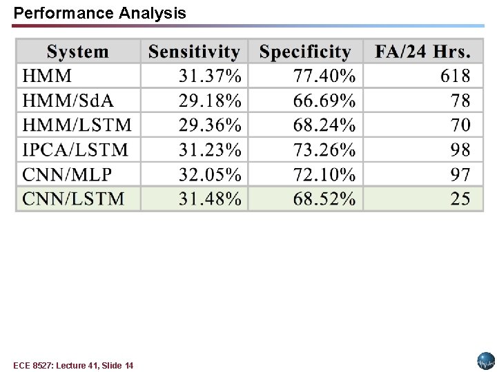
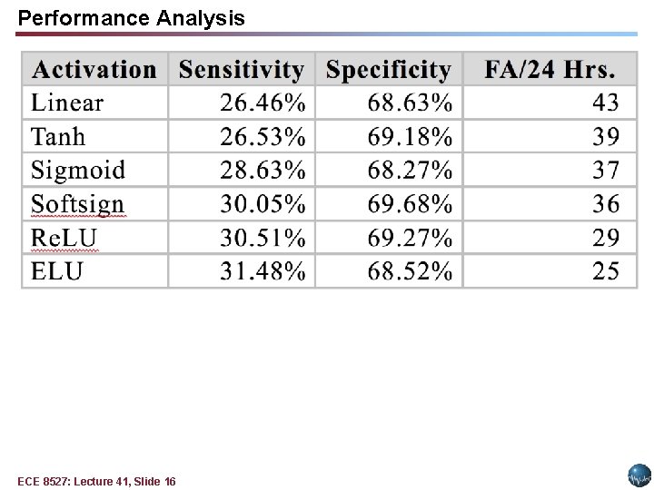
Performance Analysis ECE 8527: Lecture 41, Slide 14

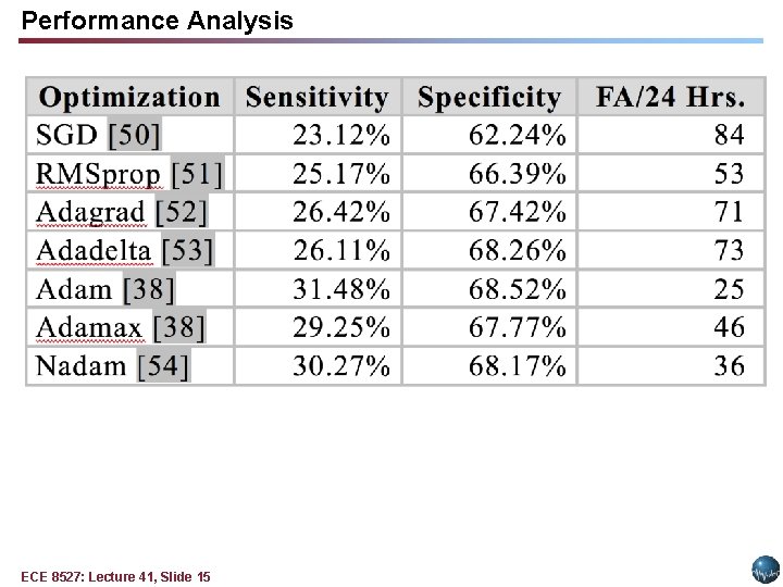
Performance Analysis ECE 8527: Lecture 41, Slide 15

Performance Analysis ECE 8527: Lecture 41, Slide 16

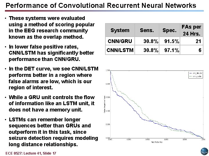
Performance of Convolutional Recurrent Neural Networks • These systems were evaluated using a method of scoring popular in the EEG research community known as the overlap method. • In lower false positive rates, CNN/LSTM has significantly better performance than CNN/GRU. • In the DET curve, we see CNN/LSTM performs better in a region where false alarms are low, which is our region of interest. • While a GRU unit controls the flow of information like an LSTM unit, it does not have a memory unit. • LSTMs can remember longer sequences better than GRUs and outperform it in this task, since seizure detection requires modeling long distance relationships. ECE 8527: Lecture 41, Slide 17 CNN/GRU 30. 8% FAs per 24 Hrs. 91. 5% 21 CNN/LSTM 30. 8% 97. 1% System Sens. Spec. 6

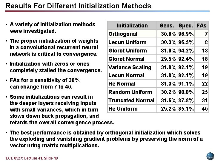
Results For Different Initialization Methods • A variety of initialization methods were investigated. • The proper initialization of weights in a convolutional recurrent neural network is critical to convergence. • Initialization with zeros or ones completely stalled the convergence. • FAs for a sensitivity of 30% can change from 7 to 40. Initialization Sens. Spec. FAs Orthogonal 30. 8% 96. 9% 7 Lecun Uniform 30. 3% 96. 5% 8 Glorot Uniform 31. 0% 94. 2% 13 Glorot Normal 29. 5% 92. 4% 18 Variance Scaling 31. 8% 92. 1% 19 Lecun Normal 31. 8% 92. 1% 19 He Normal 31. 3% 91. 1% 22 Random Uniform 30. 2% 90. 0% 25 31. 6% 87. 8% 31 29. 2% 85. 1% 40 • Some initializations can result in Truncated Normal the deeper layers receiving inputs He Uniform with small variances, which in turn slows down back propagation, and retards the overall convergence process. • The best performance is obtained by orthogonal initialization which solves the exploding and vanishing gradient problems by preserving the norm of a vector uring matrix multiplications. ECE 8527: Lecture 41, Slide 18

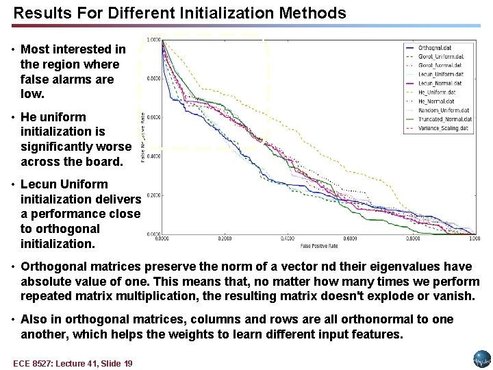
Results For Different Initialization Methods • Most interested in the region where false alarms are low. • He uniform initialization is significantly worse across the board. • Lecun Uniform initialization delivers a performance close to orthogonal initialization. • Orthogonal matrices preserve the norm of a vector nd their eigenvalues have absolute value of one. This means that, no matter how many times we perform repeated matrix multiplication, the resulting matrix doesn't explode or vanish. • Also in orthogonal matrices, columns and rows are all orthonormal to one another, which helps the weights to learn different input features. ECE 8527: Lecture 41, Slide 19

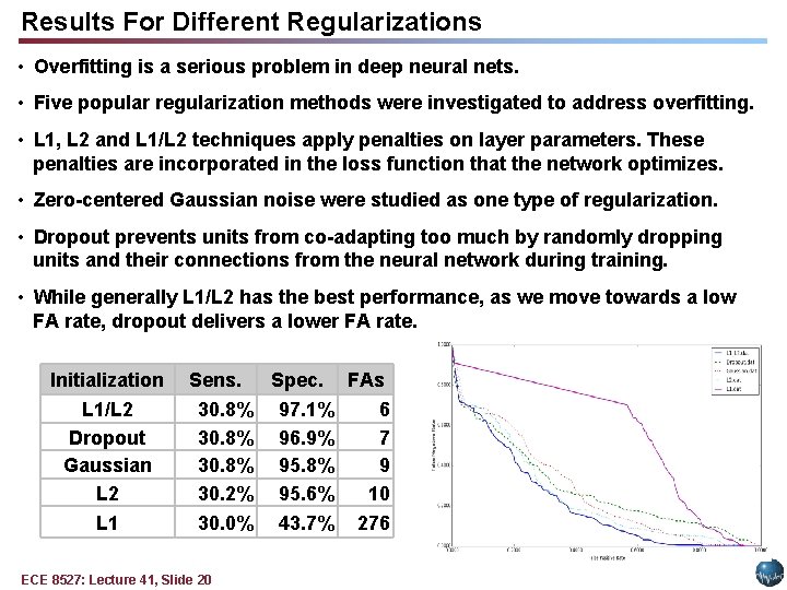
Results For Different Regularizations • Overfitting is a serious problem in deep neural nets. • Five popular regularization methods were investigated to address overfitting. • L 1, L 2 and L 1/L 2 techniques apply penalties on layer parameters. These penalties are incorporated in the loss function that the network optimizes. • Zero-centered Gaussian noise were studied as one type of regularization. • Dropout prevents units from co-adapting too much by randomly dropping units and their connections from the neural network during training. • While generally L 1/L 2 has the best performance, as we move towards a low FA rate, dropout delivers a lower FA rate. Initialization L 1/L 2 Dropout Gaussian L 2 L 1 Sens. Spec. FAs 30. 8% 97. 1% 6 30. 8% 96. 9% 7 30. 8% 95. 8% 9 30. 2% 95. 6% 10 30. 0% 43. 7% 276 ECE 8527: Lecture 41, Slide 20

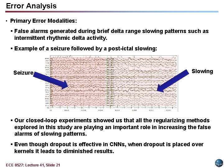
Error Analysis • Primary Error Modalities: § False alarms generated during brief delta range slowing patterns such as intermittent rhythmic delta activity. § Example of a seizure followed by a post-ictal slowing: Seizure Slowing § Our closed-loop experiments showed us that all the regularizing methods explored in this study are playing an important role in increasing the false alarms of slowing patterns. § Even though dropout is effective in CNNs, when dropout is placed over kernels it leads to diminished results. ECE 8527: Lecture 41, Slide 21

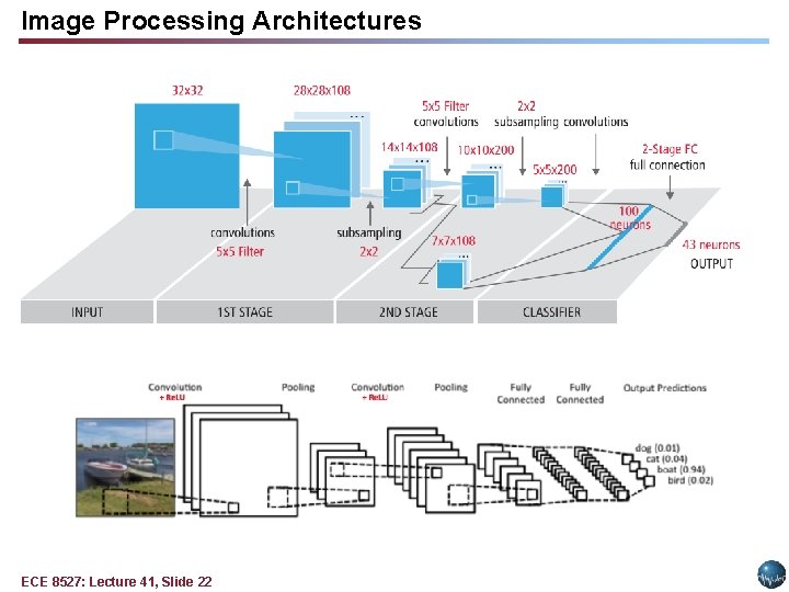
Image Processing Architectures ECE 8527: Lecture 41, Slide 22

Summary and Future Directions • Summary: § Convolutional Neural Networks are popular front ends to encode temporal and spatial correlations. § CNN/LSTM is a popular combination for many signal processing applications because LSTM has a separate memory cell and remembers longer sequences better than many architectures. § Orthogonal initialization provided the best performance because it handles the exploding and vanishing gradient problems. • Future Directions: § Robust training procedures are needed to make this technology relevant to a wide range of healthcare applications. ECE 8527: Lecture 41, Slide 23