ECE 8527 to Machine Learning and Pattern Recognition

ECE 8527 to Machine Learning and Pattern Recognition 8443 – Introduction Pattern Recognition LECTURE 01: COURSE OVERVIEW • Objectives: Terminology The Design Cycle Generalization and Risk The Bayesian Approach • Resources: Syllabus Internet Books and Notes D. H. S: Chapter 1 Glossary

Terminology • Pattern Recognition: “the act of taking raw data and taking an action based on the category of the pattern. ” • Common Applications: speech recognition, fingerprint identification (biometrics), DNA sequence identification • Related Terminology: § Machine Learning: The ability of a machine to improve its performance based on previous results. § Machine Understanding: acting on the intentions of the user generating the data. • Related Fields: artificial intelligence, signal processing and discipline-specific research (e. g. , target recognition, speech recognition, natural language processing). ECE 8527: Lecture 01, Slide 1

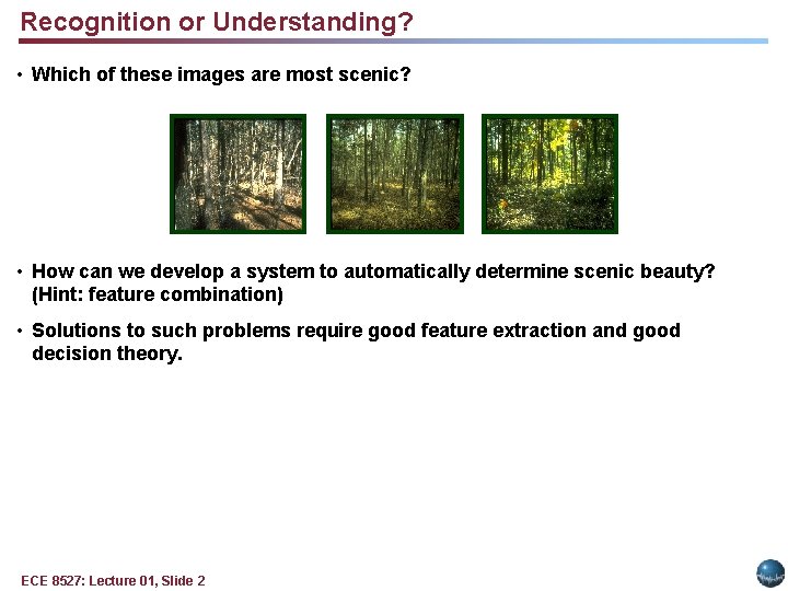
Recognition or Understanding? • Which of these images are most scenic? • How can we develop a system to automatically determine scenic beauty? (Hint: feature combination) • Solutions to such problems require good feature extraction and good decision theory. ECE 8527: Lecture 01, Slide 2

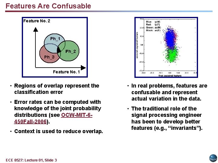
Features Are Confusable • Regions of overlap represent the classification error • Error rates can be computed with knowledge of the joint probability distributions (see OCW-MIT-6450 Fall-2006). • Context is used to reduce overlap. ECE 8527: Lecture 01, Slide 3 • In real problems, features are confusable and represent actual variation in the data. • The traditional role of the signal processing engineer has been to develop better features (e. g. , “invariants”).

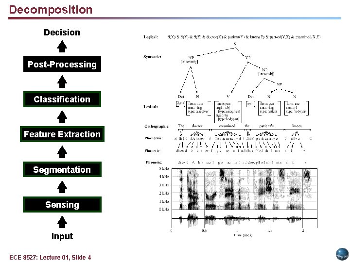
Decomposition Decision Post-Processing Classification Feature Extraction Segmentation Sensing Input ECE 8527: Lecture 01, Slide 4

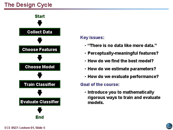
The Design Cycle Start Collect Data Key issues: Choose Features • “There is no data like more data. ” • Perceptually-meaningful features? • How do we find the best model? Choose Model • How do we estimate parameters? • How do we evaluate performance? Train Classifier Evaluate Classifier End ECE 8527: Lecture 01, Slide 5 Goal of the course: • Introduce you to mathematically rigorous ways to train and evaluate models.

Common Mistakes • I got 100% accuracy on. . . § Almost any algorithm works some of the time, but few real-world problems have ever been completely solved. § Training on the evaluation data is forbidden. § Once you use evaluation data, you should discard it. • My algorithm is better because. . . § Statistical significance and experimental design play a big role in determining the validity of a result. § There is always some probability a random choice of an algorithm will produce a better result. • Hence, in this course, we will also learn how to evaluate algorithms. ECE 8527: Lecture 01, Slide 6

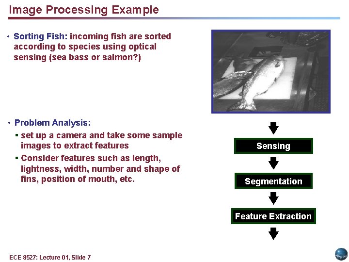
Image Processing Example • Sorting Fish: incoming fish are sorted according to species using optical sensing (sea bass or salmon? ) • Problem Analysis: § set up a camera and take some sample images to extract features § Consider features such as length, lightness, width, number and shape of fins, position of mouth, etc. Sensing Segmentation Feature Extraction ECE 8527: Lecture 01, Slide 7

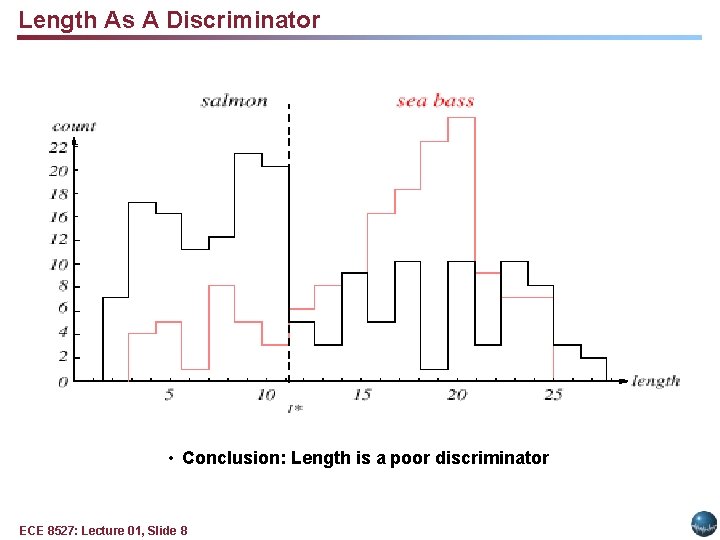
Length As A Discriminator • Conclusion: Length is a poor discriminator ECE 8527: Lecture 01, Slide 8

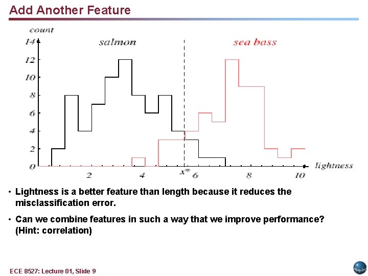
Add Another Feature • Lightness is a better feature than length because it reduces the misclassification error. • Can we combine features in such a way that we improve performance? (Hint: correlation) ECE 8527: Lecture 01, Slide 9

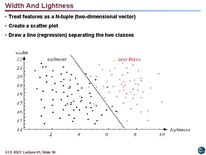
Width And Lightness • Treat features as a N-tuple (two-dimensional vector) • Create a scatter plot • Draw a line (regression) separating the two classes ECE 8527: Lecture 01, Slide 10

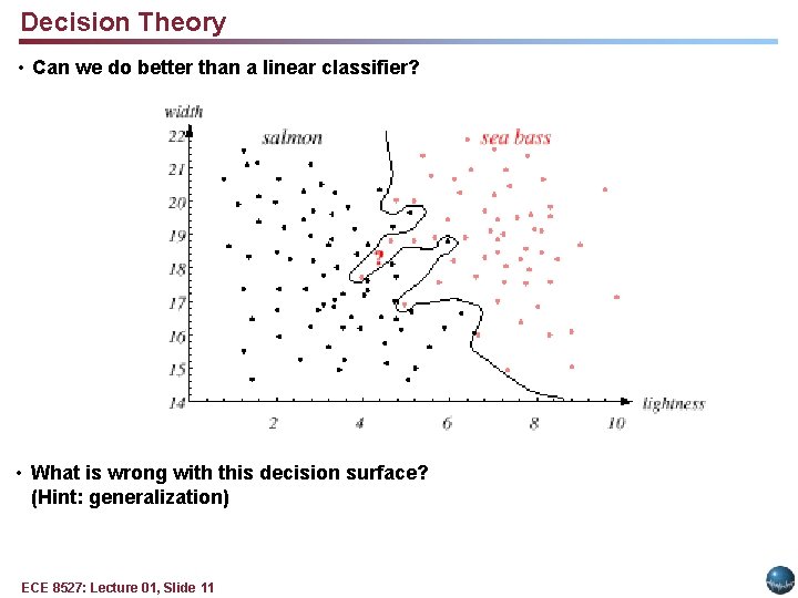
Decision Theory • Can we do better than a linear classifier? • What is wrong with this decision surface? (Hint: generalization) ECE 8527: Lecture 01, Slide 11

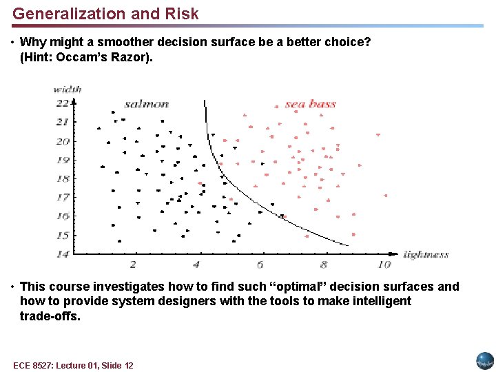
Generalization and Risk • Why might a smoother decision surface be a better choice? (Hint: Occam’s Razor). • This course investigates how to find such “optimal” decision surfaces and how to provide system designers with the tools to make intelligent trade-offs. ECE 8527: Lecture 01, Slide 12

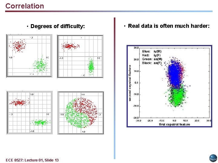
Correlation • Degrees of difficulty: ECE 8527: Lecture 01, Slide 13 • Real data is often much harder:

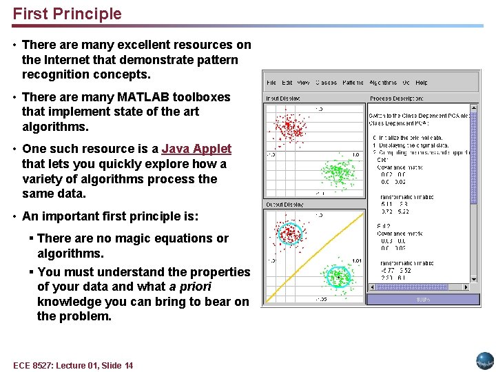
First Principle • There are many excellent resources on the Internet that demonstrate pattern recognition concepts. • There are many MATLAB toolboxes …. that implement state of the art algorithms. • One such resource is a Java Applet that lets you quickly explore how a variety of algorithms process the same data. • An important first principle is: § There are no magic equations or algorithms. § You must understand the properties of your data and what a priori knowledge you can bring to bear on the problem. ECE 8527: Lecture 01, Slide 14

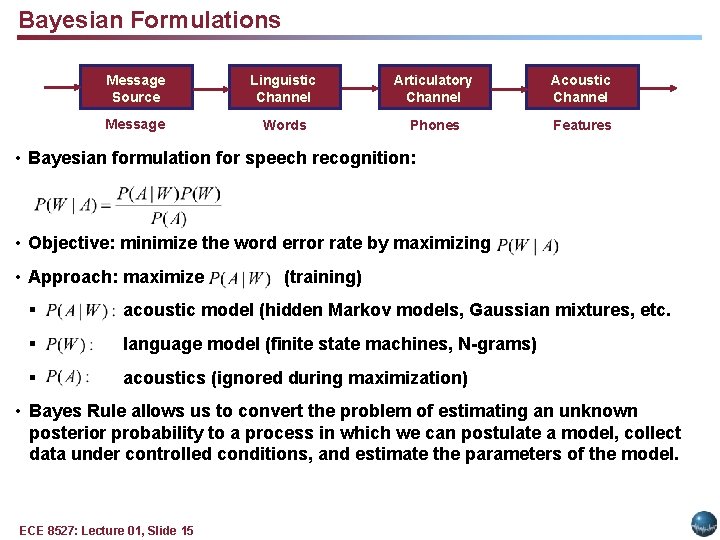
Bayesian Formulations Message Source Linguistic Channel Articulatory Channel Acoustic Channel Message Words Phones Features • Bayesian formulation for speech recognition: • Objective: minimize the word error rate by maximizing • Approach: maximize (training) § acoustic model (hidden Markov models, Gaussian mixtures, etc. § language model (finite state machines, N-grams) § acoustics (ignored during maximization) • Bayes Rule allows us to convert the problem of estimating an unknown posterior probability to a process in which we can postulate a model, collect data under controlled conditions, and estimate the parameters of the model. ECE 8527: Lecture 01, Slide 15

Summary • Pattern recognition vs. machine learning vs. machine understanding • First principle of pattern recognition? • We will focus more on decision theory and less on feature extraction. • This course emphasizes statistical and data-driven methods for optimizing system design and parameter values. • Second most important principle? ECE 8527: Lecture 01, Slide 16

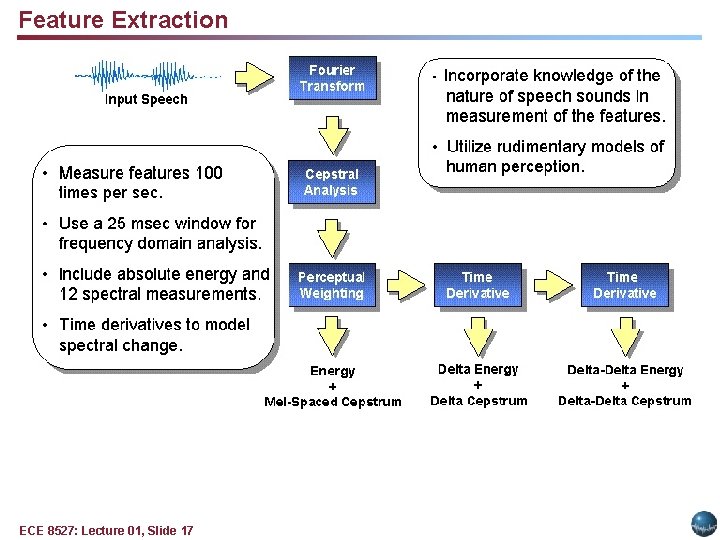
Feature Extraction ECE 8527: Lecture 01, Slide 17

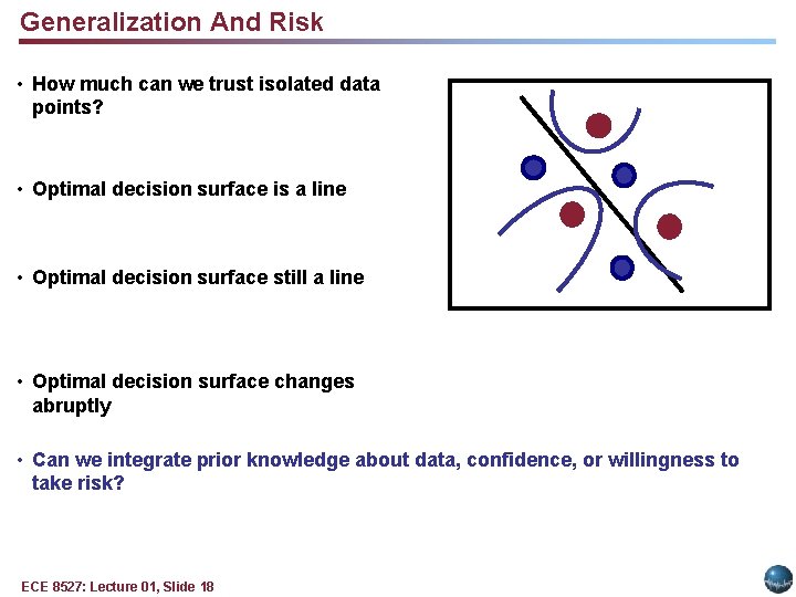
Generalization And Risk • How much can we trust isolated data points? • Optimal decision surface is a line • Optimal decision surface still a line • Optimal decision surface changes abruptly • Can we integrate prior knowledge about data, confidence, or willingness to take risk? ECE 8527: Lecture 01, Slide 18

Review • Normal (Gaussian) Distributions • Multivariate Normal (Gaussian) Distributions • Support Regions: a convenient visualization tool ECE 8527: Lecture 01, Slide 19

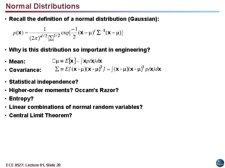
Normal Distributions • Recall the definition of a normal distribution (Gaussian): • Why is this distribution so important in engineering? • Mean: • Covariance: • • • Statistical independence? Higher-order moments? Occam’s Razor? Entropy? Linear combinations of normal random variables? Central Limit Theorem? ECE 8527: Lecture 01, Slide 20

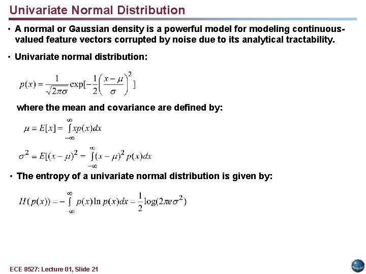
Univariate Normal Distribution • A normal or Gaussian density is a powerful model for modeling continuousvalued feature vectors corrupted by noise due to its analytical tractability. • Univariate normal distribution: where the mean and covariance are defined by: • The entropy of a univariate normal distribution is given by: ECE 8527: Lecture 01, Slide 21

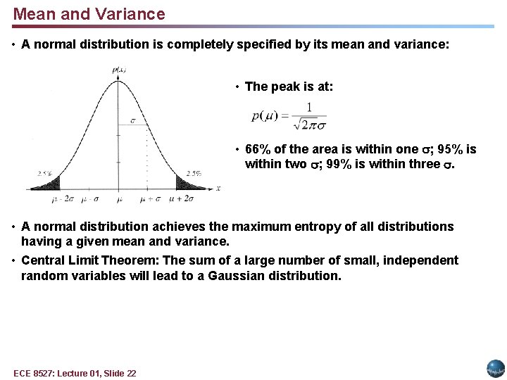
Mean and Variance • A normal distribution is completely specified by its mean and variance: • The peak is at: • 66% of the area is within one ; 95% is within two ; 99% is within three . • A normal distribution achieves the maximum entropy of all distributions having a given mean and variance. • Central Limit Theorem: The sum of a large number of small, independent random variables will lead to a Gaussian distribution. ECE 8527: Lecture 01, Slide 22

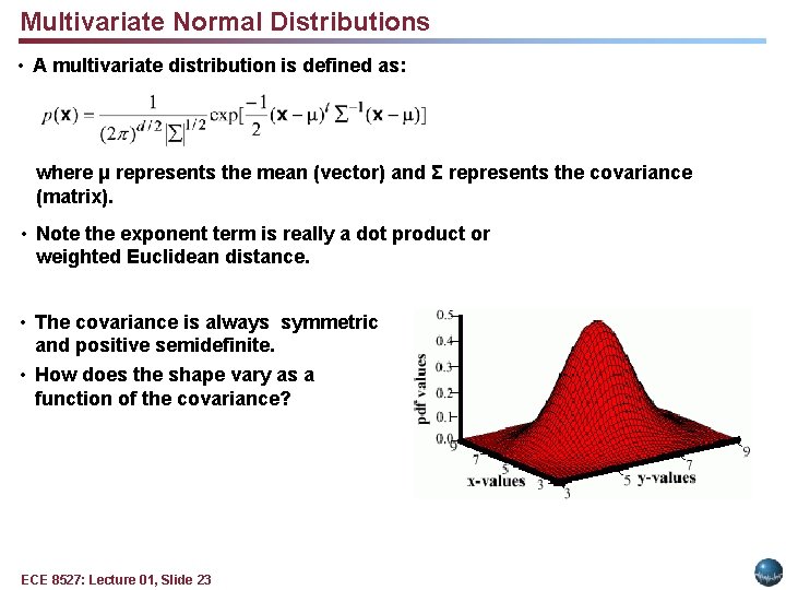
Multivariate Normal Distributions • A multivariate distribution is defined as: where μ represents the mean (vector) and Σ represents the covariance (matrix). • Note the exponent term is really a dot product or weighted Euclidean distance. • The covariance is always symmetric and positive semidefinite. • How does the shape vary as a function of the covariance? ECE 8527: Lecture 01, Slide 23

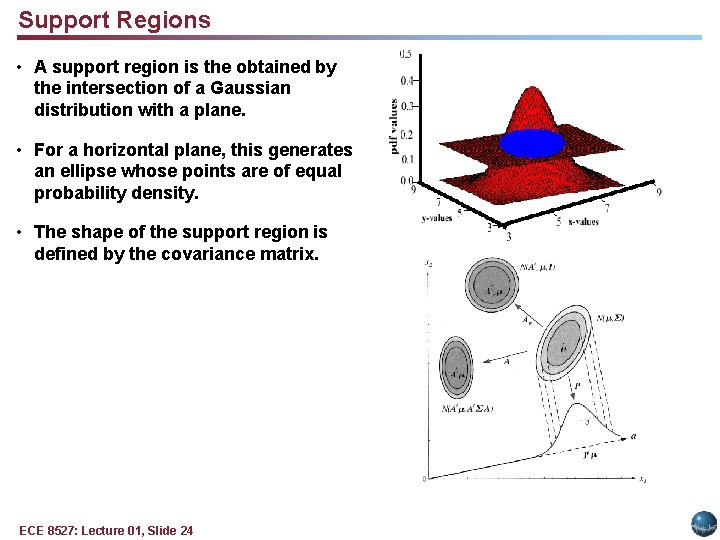
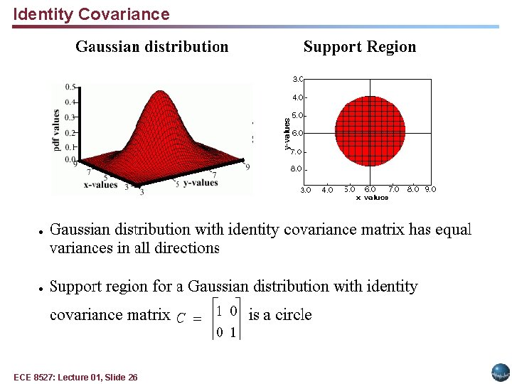
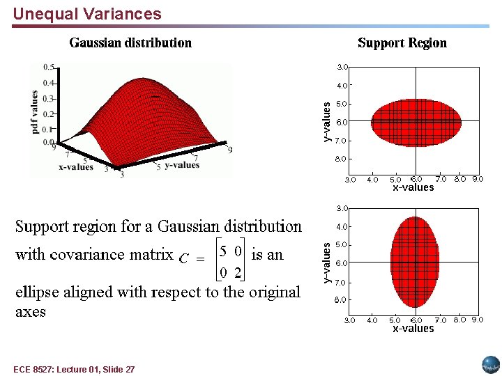
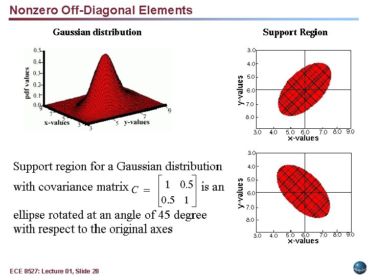
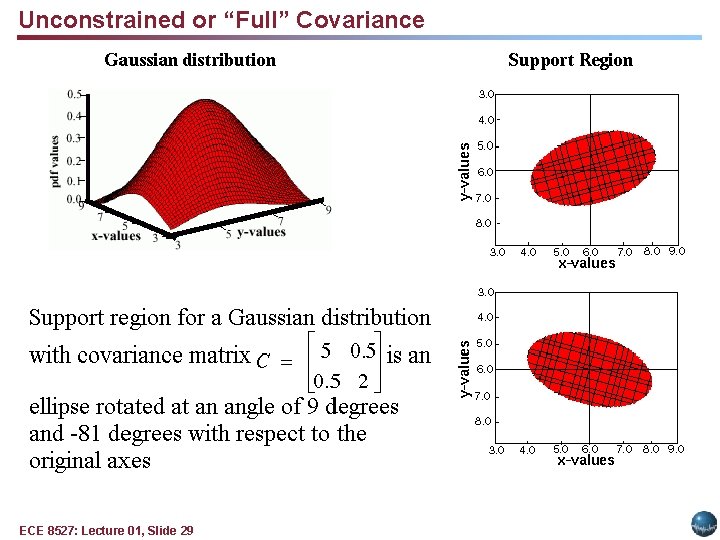
Support Regions • A support region is the obtained by the intersection of a Gaussian distribution with a plane. • For a horizontal plane, this generates an ellipse whose points are of equal probability density. • The shape of the support region is defined by the covariance matrix. ECE 8527: Lecture 01, Slide 24

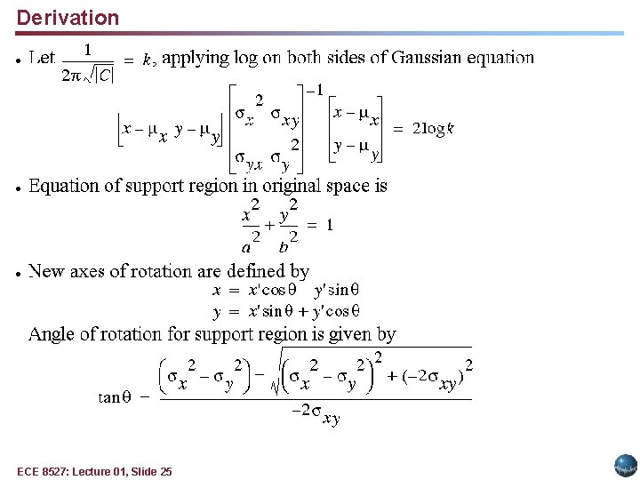
Derivation ECE 8527: Lecture 01, Slide 25

Identity Covariance ECE 8527: Lecture 01, Slide 26

Unequal Variances ECE 8527: Lecture 01, Slide 27

Nonzero Off-Diagonal Elements ECE 8527: Lecture 01, Slide 28

Unconstrained or “Full” Covariance ECE 8527: Lecture 01, Slide 29