ECE 8443 Pattern Recognition LECTURE 24 NETWORKS MAPS

ECE 8443 – Pattern Recognition LECTURE 24: NETWORKS, MAPS AND CLUSTERING • Objectives: Validity On-Line Clustering Adaptive Resonance Graph Theoretic Methods Nonlinear Component Analysis Multidimensional Scaling Self-Organizing Maps Dimensionality Reduction • Resources: M. H. : Cluster Validity Wiki: Adaptive Resonance Theory J. A. : Graph Theoretic Methods E. M. : Nonlinear Component Analysis F. Y. : Multidimensional Scaling URL: Audio:

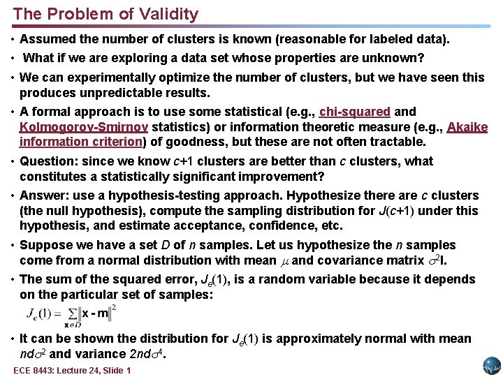
The Problem of Validity • Assumed the number of clusters is known (reasonable for labeled data). • What if we are exploring a data set whose properties are unknown? • We can experimentally optimize the number of clusters, but we have seen this produces unpredictable results. • A formal approach is to use some statistical (e. g. , chi-squared and Kolmogorov-Smirnov statistics) or information theoretic measure (e. g. , Akaike information criterion) of goodness, but these are not often tractable. • Question: since we know c+1 clusters are better than c clusters, what constitutes a statistically significant improvement? • Answer: use a hypothesis-testing approach. Hypothesize there are c clusters (the null hypothesis), compute the sampling distribution for J(c+1) under this hypothesis, and estimate acceptance, confidence, etc. • Suppose we have a set D of n samples. Let us hypothesize the n samples come from a normal distribution with mean and covariance matrix 2 I. • The sum of the squared error, Je(1), is a random variable because it depends on the particular set of samples: • It can be shown the distribution for Je(1) is approximately normal with mean nd 2 and variance 2 nd 4. ECE 8443: Lecture 24, Slide 1

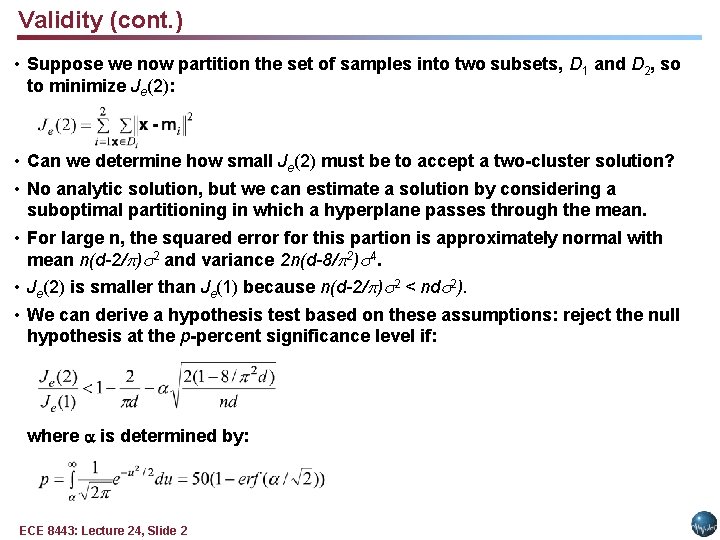
Validity (cont. ) • Suppose we now partition the set of samples into two subsets, D 1 and D 2, so to minimize Je(2): • Can we determine how small Je(2) must be to accept a two-cluster solution? • No analytic solution, but we can estimate a solution by considering a suboptimal partitioning in which a hyperplane passes through the mean. • For large n, the squared error for this partion is approximately normal with mean n(d-2/ ) 2 and variance 2 n(d-8/ 2) 4. • Je(2) is smaller than Je(1) because n(d-2/ ) 2 < nd 2). • We can derive a hypothesis test based on these assumptions: reject the null hypothesis at the p-percent significance level if: where is determined by: ECE 8443: Lecture 24, Slide 2

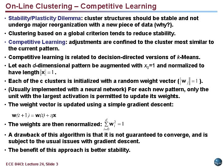
On-Line Clustering – Competitive Learning • Stability/Plasticity Dilemma: cluster structures should be stable and not undergo major reorganization with a new piece of data (why? ). • Clustering based on a global criterion tends to reduce stability. • Competitive Learning: adjustments are confined to the cluster most similar to the current pattern. • Competitive learning is related to decision-directed versions of k-Means. • Let each d-dimensional pattern be augmented with x 0=1 and normalized to have length. • Each of the c clusters is initialized with a random weight vector ( ). • (Usually implemented with a neural network) For each new pattern, only the unit with the largest activation is permitted to update its weights. • The weight vector is updated using a simple gradient descent: • The weights are then renormalized: • A drawback of this algorithm is that it is not guaranteed to converge, and is subject to the usual issues with gradient descent. • The benefit of this approach is better stability. ECE 8443: Lecture 24, Slide 3

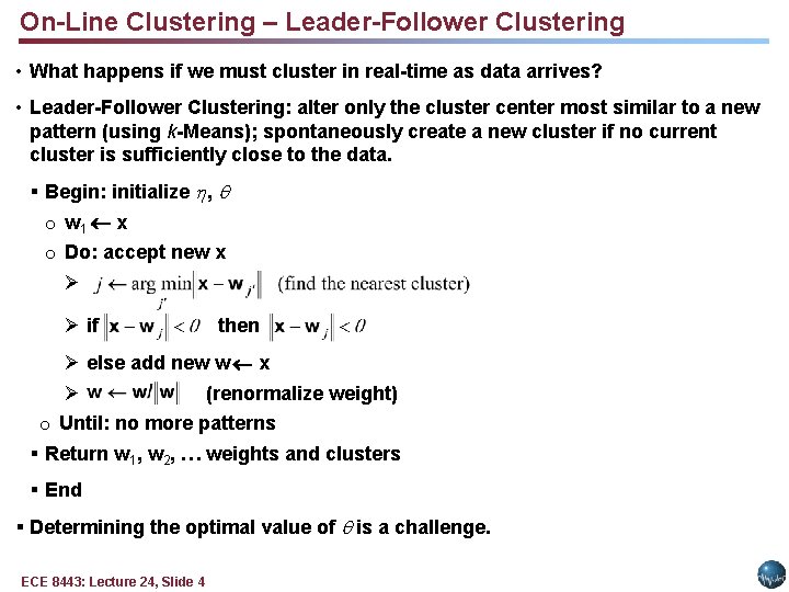
On-Line Clustering – Leader-Follower Clustering • What happens if we must cluster in real-time as data arrives? • Leader-Follower Clustering: alter only the cluster center most similar to a new pattern (using k-Means); spontaneously create a new cluster if no current cluster is sufficiently close to the data. § Begin: initialize , o w 1 x o Do: accept new x Ø Ø if then Ø else add new w x Ø (renormalize weight) o Until: no more patterns § Return w 1, w 2, … weights and clusters § End § Determining the optimal value of is a challenge. ECE 8443: Lecture 24, Slide 4

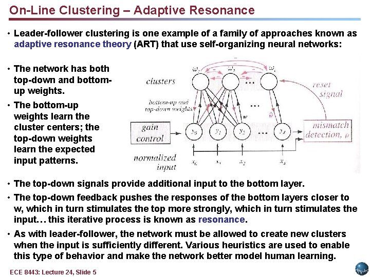
On-Line Clustering – Adaptive Resonance • Leader-follower clustering is one example of a family of approaches known as adaptive resonance theory (ART) that use self-organizing neural networks: • The network has both top-down and bottomup weights. • The bottom-up weights learn the cluster centers; the top-down weights learn the expected input patterns. • The top-down signals provide additional input to the bottom layer. • The top-down feedback pushes the responses of the bottom layers closer to w, which in turn stimulates the top more strongly, which in turn stimulates the input… this iterative process is known as resonance. • As with leader-follower, the network must be allowed to create new clusters when the input is sufficiently different. Various heuristics are used to enable this type of behavior and make the network better model human learning. ECE 8443: Lecture 24, Slide 5

Graph Theoretic Methods • Pick a threshold, s 0, and decide xi is similar to xj if s(xi, xj) > s 0. • This matrix induces a similarity graph in which nodes correspond to points and an edge joins node i and node j if and only if sij > 0. • The clusterings produced by single linkage algorithms and by a modified version of the complete-linkage algorithm can be described in terms of this similarity graph. • There are many graphical methods designed to represent the similarity graph with reduced complexity. • With a single linkage algorithm, two samples are in the same cluster if and only If there exists a chain x, x 1, x 2, , , xk, x’ such that x is similar to x 1, x 1 is similar to x 2, … • With a complete linkage algorithm, all samples in a given cluster must be similar to one another and no sample can be in more than one cluster. • A nearest neighbor algorithm can be viewed as an algorithm for finding a minimum spanning tree. • Other clustering algorithms can be viewed in terms of these graphs. • A figure of merit for such graphs is the edge length distribution. ECE 8443: Lecture 24, Slide 6

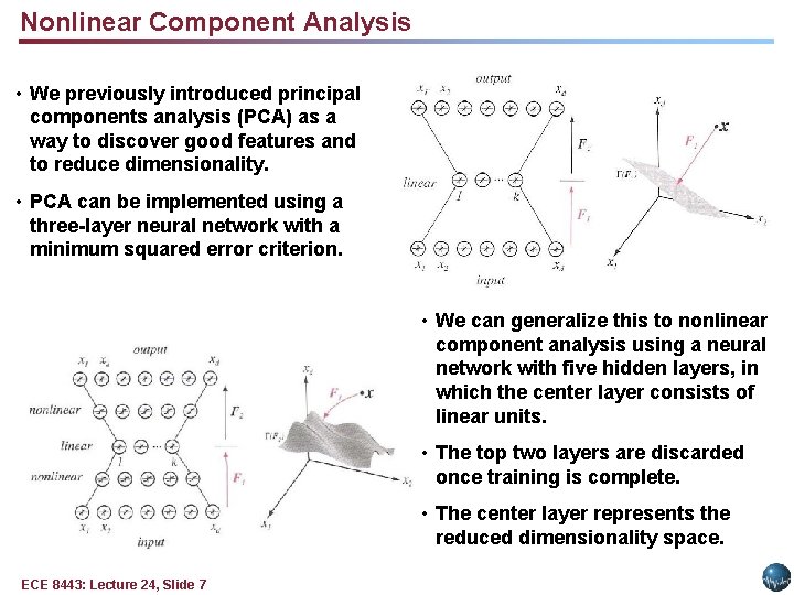
Nonlinear Component Analysis • We previously introduced principal components analysis (PCA) as a way to discover good features and to reduce dimensionality. • PCA can be implemented using a three-layer neural network with a minimum squared error criterion. • We can generalize this to nonlinear component analysis using a neural network with five hidden layers, in which the center layer consists of linear units. • The top two layers are discarded once training is complete. • The center layer represents the reduced dimensionality space. ECE 8443: Lecture 24, Slide 7

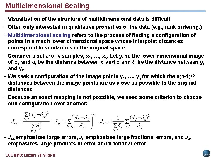
Multidimensional Scaling • Visualization of the structure of multidimensional data is difficult. • Often only interested in qualitative properties of the data (e. g. , rank ordering. ) • Multidimensional scaling refers to the process of finding a configuration of points in a much lower dimensional space whose interpoint distances correspond to similarities in the original space. • Consider a set D of n samples, x 1, …, xn. Let yi be the lower dimensional image of xi, and dij be the distance between xi and xj and ij be the distance between yi and yj. • We seek a configuration of the image points y 1, …, yn for which the n(n-1)/2 distances between the image points are as close as possible to the original distances. • Because an exact mapping is not possible, we need some criterion to choose one configuration over another: • Jee emphasizes large errors, Jff emphasizes large fractional errors, and Jef emphasizes large products of error and fractional error. ECE 8443: Lecture 24, Slide 8

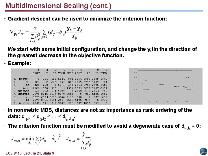
Multidimensional Scaling (cont. ) • Gradient descent can be used to minimize the criterion function: We start with some initial configuration, and change the yi Iin the direction of the greatest decrease in the objective function. • Example: • In nonmetric MDS, distances are not as importance as rank ordering of the data: di 1, j 1 di 2, j 2 … dim, jm. • The criterion function must be modified to avoid a degenerate case of di 1, j 1 = 0: ECE 8443: Lecture 24, Slide 9

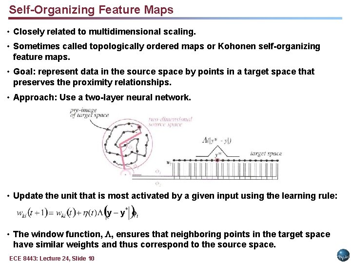
Self-Organizing Feature Maps • Closely related to multidimensional scaling. • Sometimes called topologically ordered maps or Kohonen self-organizing feature maps. • Goal: represent data in the source space by points in a target space that preserves the proximity relationships. • Approach: Use a two-layer neural network. • Update the unit that is most activated by a given input using the learning rule: • The window function, , ensures that neighboring points in the target space have similar weights and thus correspond to the source space. ECE 8443: Lecture 24, Slide 10

Summary • Introduced the problem of validity. • Derived a hypothesis test to determine if a new clustering produces a statistically significant better result. • Introduced competitive learning, leader-follower clustering, and adaptive resonance theory. • Described applications of graph theoretic methods to clustering. • Introduced nonlinear component analysis. • Introduced multidimensional scaling. • Introduced self-organizing feature maps. ECE 8443: Lecture 24, Slide 11