ECE 8443 Pattern Recognition LECTURE 10 MAXIMUM LIKELIHOOD

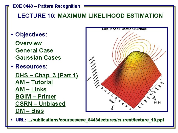
ECE 8443 – Pattern Recognition LECTURE 10: MAXIMUM LIKELIHOOD ESTIMATION • Objectives: Overview General Case Gaussian Cases • Resources: DHS – Chap. 3 (Part 1) AM – Tutorial AM – Links BGIM – Primer CSRN – Unbiased DM – Bias • URL: . . . /publications/courses/ece_8443/lectures/current/lecture_10. ppt

10: MAXIMUM LIKELIHOOD ESTIMATION INTRODUCTION • In Chapter 2, we learned how to design an optimal classifier if we knew the prior probabilities, P( i), and class-conditional densities, p(x| i). • What can we do if we do not have this information? • What limitations do we face? • There are two common approaches to parameter estimation: maximum-likelihood and Bayesian estimation. • Maximum likelihood: treat the parameters as quantities whose values are fixed but unknown. • Bayes: treat the parameters as random variables having some known prior distribution. Observations of samples converts this to a posterior. • Bayesian learning: sharpen the a posteriori density causing it to peak near the true value.

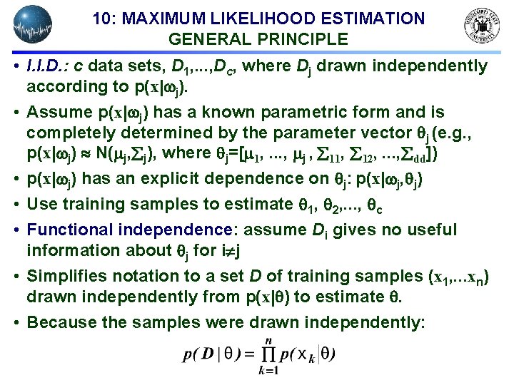
10: MAXIMUM LIKELIHOOD ESTIMATION GENERAL PRINCIPLE • I. I. D. : c data sets, D 1, . . . , Dc, where Dj drawn independently according to p(x| j). • Assume p(x| j) has a known parametric form and is completely determined by the parameter vector j (e. g. , p(x| j) N( j, j), where j=[ 1, . . . , j , 11, 12, . . . , dd]) • p(x| j) has an explicit dependence on j: p(x| j, j) • Use training samples to estimate 1, 2, . . . , c • Functional independence: assume Di gives no useful information about j for i j • Simplifies notation to a set D of training samples (x 1, . . . xn) drawn independently from p(x| ) to estimate . • Because the samples were drawn independently:

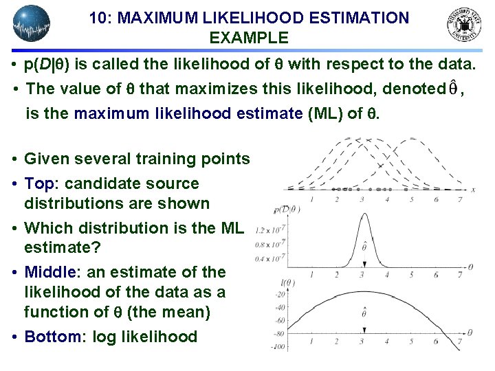
10: MAXIMUM LIKELIHOOD ESTIMATION EXAMPLE • p(D| ) is called the likelihood of with respect to the data. • The value of that maximizes this likelihood, denoted , is the maximum likelihood estimate (ML) of . • Given several training points • Top: candidate source distributions are shown • Which distribution is the ML estimate? • Middle: an estimate of the likelihood of the data as a function of (the mean) • Bottom: log likelihood

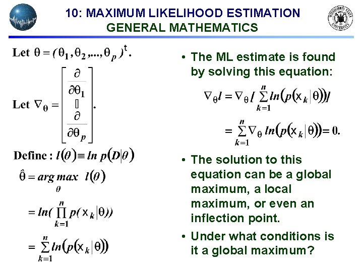
10: MAXIMUM LIKELIHOOD ESTIMATION GENERAL MATHEMATICS • The ML estimate is found by solving this equation: • The solution to this equation can be a global maximum, a local maximum, or even an inflection point. • Under what conditions is it a global maximum?

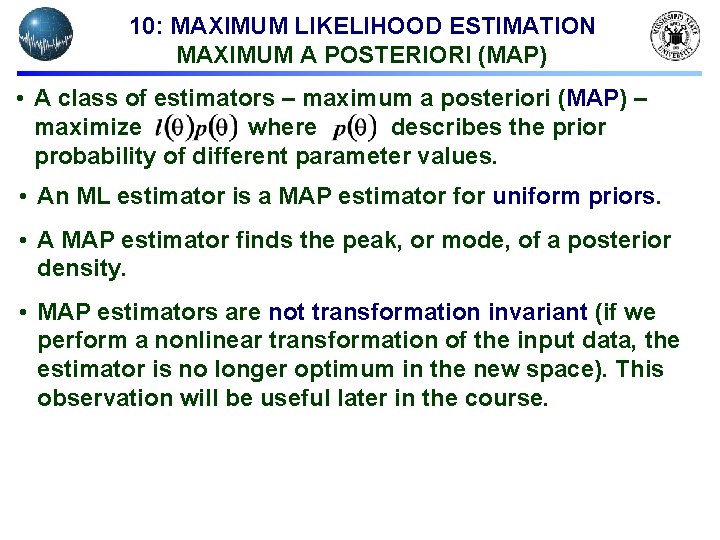
10: MAXIMUM LIKELIHOOD ESTIMATION MAXIMUM A POSTERIORI (MAP) • A class of estimators – maximum a posteriori (MAP) – maximize where describes the prior probability of different parameter values. • An ML estimator is a MAP estimator for uniform priors. • A MAP estimator finds the peak, or mode, of a posterior density. • MAP estimators are not transformation invariant (if we perform a nonlinear transformation of the input data, the estimator is no longer optimum in the new space). This observation will be useful later in the course.

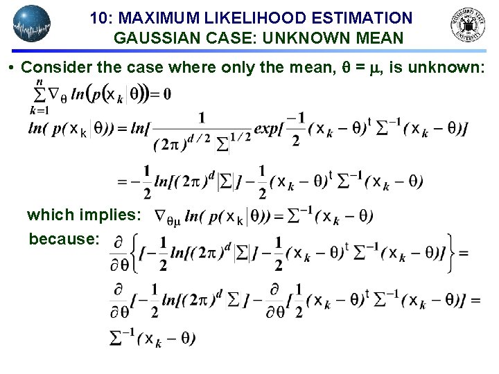
10: MAXIMUM LIKELIHOOD ESTIMATION GAUSSIAN CASE: UNKNOWN MEAN • Consider the case where only the mean, = , is unknown: which implies: because:

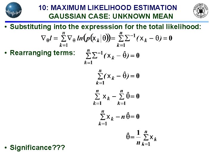
10: MAXIMUM LIKELIHOOD ESTIMATION GAUSSIAN CASE: UNKNOWN MEAN • Substituting into the expresssion for the total likelihood: • Rearranging terms: • Significance? ? ?

10: MAXIMUM LIKELIHOOD ESTIMATION UNKNOWN MEAN AND VARIANCE • Let = [ , 2]: • The full likelihood leads to:

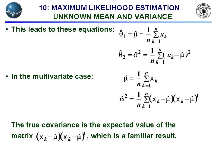
10: MAXIMUM LIKELIHOOD ESTIMATION UNKNOWN MEAN AND VARIANCE • This leads to these equations: • In the multivariate case: The true covariance is the expected value of the matrix , which is a familiar result.

10: MAXIMUM LIKELIHOOD ESTIMATION CONVERGENCE OF THE MEAN • Does the maximum likelihood estimate of the variance converge to the true value of the variance? Let’s start with a few simple results we will need later. • Expected value of the ML estimate of the mean:

10: MAXIMUM LIKELIHOOD ESTIMATION VARIANCE OF ML ESTIMATE OF THE MEAN • The expected value of xixj will be 2 for j k since the two random variables are independent. • The expected value of xi 2 will be 2 + 2. • Hence, in the summation above, we have n 2 -n terms with expected value 2 and n terms with expected value 2 + 2. • Thus, which implies: • We see that the variance of the estimate goes to zero as n goes to infinity, and our estimate converges to the true estimate (error goes to zero).

10: MAXIMUM LIKELIHOOD ESTIMATION VARIANCE RELATIONSHIPS • We will need one more result: Note that this implies: • Now we can combine these results. Recall our expression for the ML estimate of the variance:

10: MAXIMUM LIKELIHOOD ESTIMATION COVARIANCE EXPANSION • Expand the covariance and simplify: • One more intermediate term to derive:

10: MAXIMUM LIKELIHOOD ESTIMATION BIASED VARIANCE ESTIMATE • Substitute our previously derived expression for the second term:

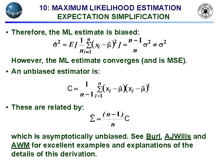
10: MAXIMUM LIKELIHOOD ESTIMATION EXPECTATION SIMPLIFICATION • Therefore, the ML estimate is biased: However, the ML estimate converges (and is MSE). • An unbiased estimator is: • These are related by: which is asymptotically unbiased. See Burl, AJWills and AWM for excellent examples and explanations of the details of this derivation.