ECE 8423 8443Adaptive Pattern Recognition ECE Signal Processing

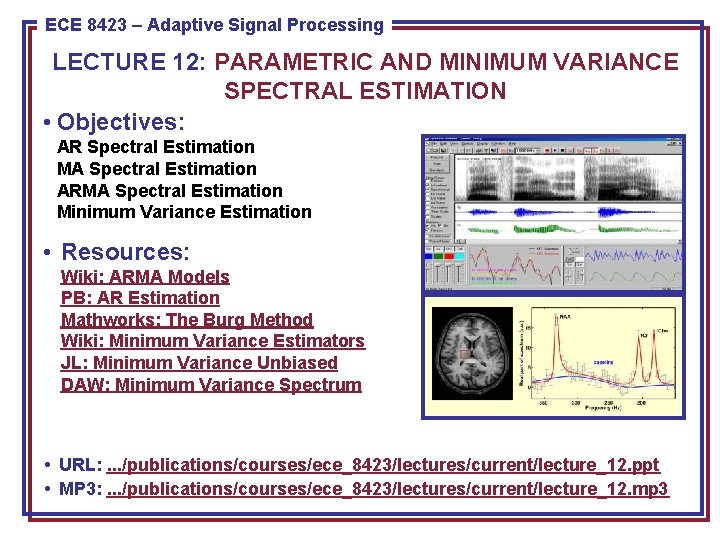
ECE 8423 8443––Adaptive Pattern Recognition ECE Signal Processing LECTURE 12: PARAMETRIC AND MINIMUM VARIANCE SPECTRAL ESTIMATION • Objectives: AR Spectral Estimation MA Spectral Estimation ARMA Spectral Estimation Minimum Variance Estimation • Resources: Wiki: ARMA Models PB: AR Estimation Mathworks: The Burg Method Wiki: Minimum Variance Estimators JL: Minimum Variance Unbiased DAW: Minimum Variance Spectrum • URL: . . . /publications/courses/ece_8423/lectures/current/lecture_12. ppt • MP 3: . . . /publications/courses/ece_8423/lectures/current/lecture_12. mp 3

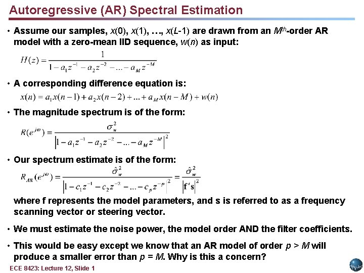
Autoregressive (AR) Spectral Estimation • Assume our samples, x(0), x(1), …, x(L-1) are drawn from an Mth-order AR model with a zero-mean IID sequence, w(n) as input: • A corresponding difference equation is: • The magnitude spectrum is of the form: • Our spectrum estimate is of the form: where f represents the model parameters, and s is referred to as a frequency scanning vector or steering vector. • We must estimate the noise power, the model order AND the filter coefficients. • This would be easy except we know that an AR model of order p > M will produce a smaller error than p = M. Why is this a concern? ECE 8423: Lecture 12, Slide 1

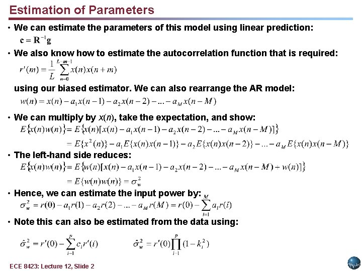
Estimation of Parameters • We can estimate the parameters of this model using linear prediction: • We also know how to estimate the autocorrelation function that is required: using our biased estimator. We can also rearrange the AR model: • We can multiply by x(n), take the expectation, and show: • The left-hand side reduces: • Hence, we can estimate the input power by: • Note this can also be estimated from the data using: ECE 8423: Lecture 12, Slide 2

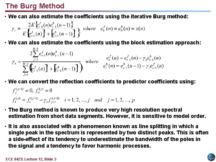
The Burg Method • We can also estimate the coefficients using the iterative Burg method: • We can also estimate the coefficients using the block estimation approach: • We can convert the reflection coefficients to predictor coefficients using: • The Burg method is known to produce very high resolution spectral estimation from short data segments. However, it is sensitive to model order. • It is also associated with a phenomenon known as line splitting in which a single peak in the spectrum is represented by two distinct peaks. This is often a side-effect of its tendency to underestimate the bandwidth of the poles in the signal and a tendency to favor harmonic processes. ECE 8423: Lecture 12, Slide 3

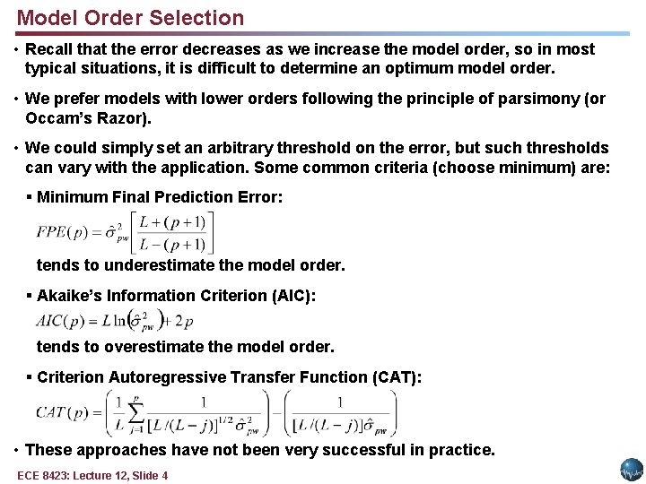
Model Order Selection • Recall that the error decreases as we increase the model order, so in most typical situations, it is difficult to determine an optimum model order. • We prefer models with lower orders following the principle of parsimony (or Occam’s Razor). • We could simply set an arbitrary threshold on the error, but such thresholds can vary with the application. Some common criteria (choose minimum) are: § Minimum Final Prediction Error: tends to underestimate the model order. § Akaike’s Information Criterion (AIC): tends to overestimate the model order. § Criterion Autoregressive Transfer Function (CAT): • These approaches have not been very successful in practice. ECE 8423: Lecture 12, Slide 4

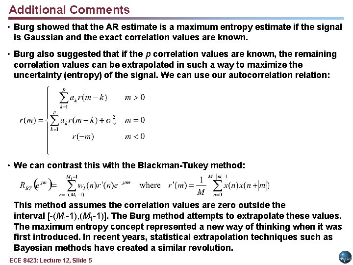
Additional Comments • Burg showed that the AR estimate is a maximum entropy estimate if the signal is Gaussian and the exact correlation values are known. • Burg also suggested that if the p correlation values are known, the remaining correlation values can be extrapolated in such a way to maximize the uncertainty (entropy) of the signal. We can use our autocorrelation: • We can contrast this with the Blackman-Tukey method: This method assumes the correlation values are zero outside the interval [-(M 1 -1), (M 1 -1)]. The Burg method attempts to extrapolate these values. The maximum entropy concept represented a new way of thinking when it was first introduced. In recent years, statistical extrapolation techniques such as Bayesian methods have created a similar revolution. ECE 8423: Lecture 12, Slide 5

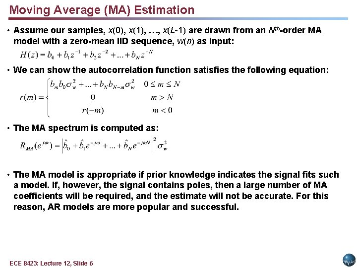
Moving Average (MA) Estimation • Assume our samples, x(0), x(1), …, x(L-1) are drawn from an Nth-order MA model with a zero-mean IID sequence, w(n) as input: • We can show the autocorrelation function satisfies the following equation: • The MA spectrum is computed as: • The MA model is appropriate if prior knowledge indicates the signal fits such a model. If, however, the signal contains poles, then a large number of MA coefficients will be required, and the estimate will not be accurate. For this reason, AR models are more popular and successful. ECE 8423: Lecture 12, Slide 6

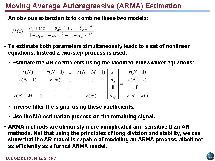
Moving Average Autoregressive (ARMA) Estimation • An obvious extension is to combine these two models: • To estimate both parameters simultaneously leads to a set of nonlinear equations. Instead a two-step process is used: § Estimate the AR coefficients using the Modified Yule-Walker equations: § Inverse filter the signal using these coefficients. § Use the MA estimation process on the remaining signal. • ARMA methods are obviously more complicated and sensitive than AR methods. Not that using the principles of long division and stability, we can show that the AR model is capable of modeling an ARMA process, albeit not as efficiently as a formal ARMA model. ECE 8423: Lecture 12, Slide 7

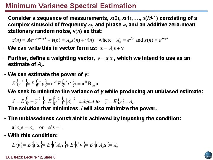
Minimum Variance Spectral Estimation • Consider a sequence of measurements, x(0), x(1), …, x(M-1) consisting of a complex sinusoid of frequency 0 and phase , and an additive zero-mean stationary random noise, v(n) so that: • We can write this in vector form as: • Further, define a weighting vector, estimate of Ac. , which we intend to use as an • We can estimate the power of y: We seek to minimize the variance of y while producing an unbiased estimate: The solution that minimizes J will also minimize the power. • The unbiasedness constraint is achieved by imposing the condition: • With this condition: ECE 8423: Lecture 12, Slide 8

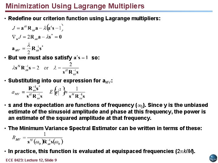
Minimization Using Lagrange Multipliers • Redefine our criterion function using Lagrange multipliers: • But we must also satisfy so: • Substituting into our expression for a. MV: • s and the expectation are functions of frequency ( 0). Since y is the unbiased estimate of the sinusoid amplitude and phase at this frequency, the power is an estimate of the squared amplitude at that frequency. • The Minimum Variance Spectral Estimator can be written in terms of these: • In practice, this function is evaluated at equispaced frequencies (2 k/M). ECE 8423: Lecture 12, Slide 9

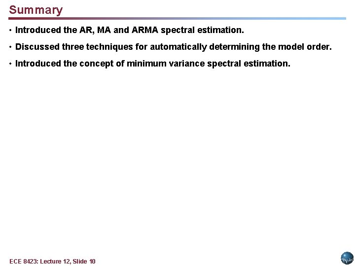
Summary • Introduced the AR, MA and ARMA spectral estimation. • Discussed three techniques for automatically determining the model order. • Introduced the concept of minimum variance spectral estimation. ECE 8423: Lecture 12, Slide 10