ECE 8423 8443Adaptive Pattern Recognition ECE Signal Processing
- Slides: 13

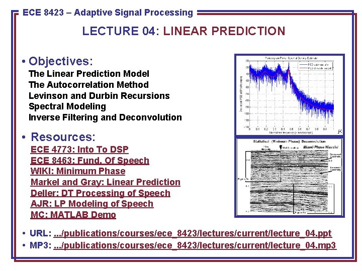
ECE 8423 8443––Adaptive Pattern Recognition ECE Signal Processing LECTURE 04: LINEAR PREDICTION • Objectives: The Linear Prediction Model The Autocorrelation Method Levinson and Durbin Recursions Spectral Modeling Inverse Filtering and Deconvolution • Resources: ECE 4773: Into To DSP ECE 8463: Fund. Of Speech WIKI: Minimum Phase Markel and Gray: Linear Prediction Deller: DT Processing of Speech AJR: LP Modeling of Speech MC: MATLAB Demo • URL: . . . /publications/courses/ece_8423/lectures/current/lecture_04. ppt • MP 3: . . . /publications/courses/ece_8423/lectures/current/lecture_04. mp 3

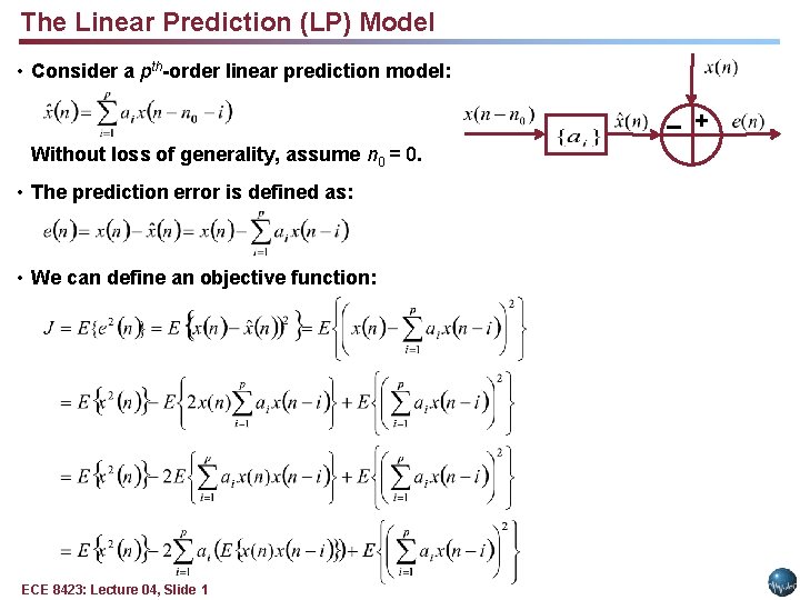
The Linear Prediction (LP) Model • Consider a pth-order linear prediction model: – + Without loss of generality, assume n 0 = 0. • The prediction error is defined as: • We can define an objective function: ECE 8423: Lecture 04, Slide 1

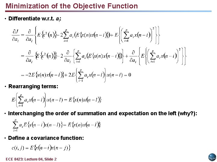
Minimization of the Objective Function • Differentiate w. r. t. al: • Rearranging terms: • Interchanging the order of summation and expectation on the left (why? ): • Define a covariance function: ECE 8423: Lecture 04, Slide 2

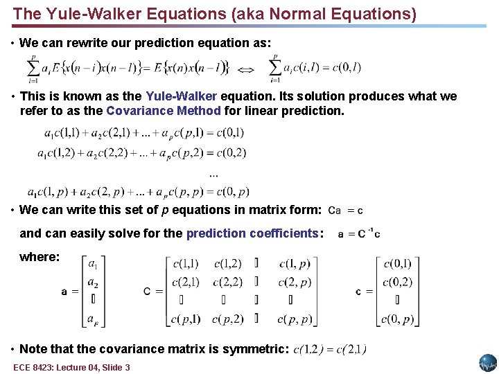
The Yule-Walker Equations (aka Normal Equations) • We can rewrite our prediction equation as: • This is known as the Yule-Walker equation. Its solution produces what we refer to as the Covariance Method for linear prediction. • We can write this set of p equations in matrix form: and can easily solve for the prediction coefficients: where: • Note that the covariance matrix is symmetric: ECE 8423: Lecture 04, Slide 3

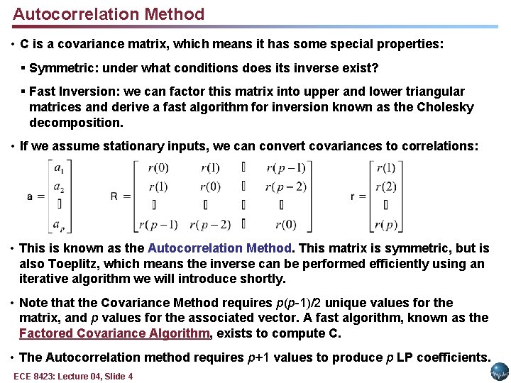
Autocorrelation Method • C is a covariance matrix, which means it has some special properties: § Symmetric: under what conditions does its inverse exist? § Fast Inversion: we can factor this matrix into upper and lower triangular matrices and derive a fast algorithm for inversion known as the Cholesky decomposition. • If we assume stationary inputs, we can convert covariances to correlations: • This is known as the Autocorrelation Method. This matrix is symmetric, but is also Toeplitz, which means the inverse can be performed efficiently using an iterative algorithm we will introduce shortly. • Note that the Covariance Method requires p(p-1)/2 unique values for the matrix, and p values for the associated vector. A fast algorithm, known as the Factored Covariance Algorithm, exists to compute C. • The Autocorrelation method requires p+1 values to produce p LP coefficients. ECE 8423: Lecture 04, Slide 4

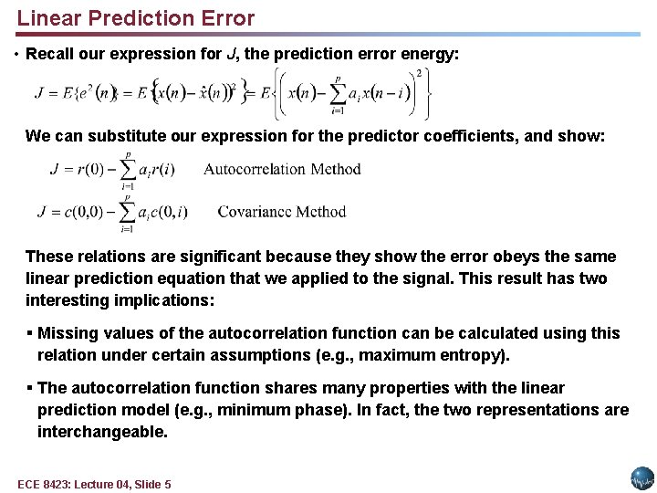
Linear Prediction Error • Recall our expression for J, the prediction error energy: We can substitute our expression for the predictor coefficients, and show: These relations are significant because they show the error obeys the same linear prediction equation that we applied to the signal. This result has two interesting implications: § Missing values of the autocorrelation function can be calculated using this relation under certain assumptions (e. g. , maximum entropy). § The autocorrelation function shares many properties with the linear prediction model (e. g. , minimum phase). In fact, the two representations are interchangeable. ECE 8423: Lecture 04, Slide 5

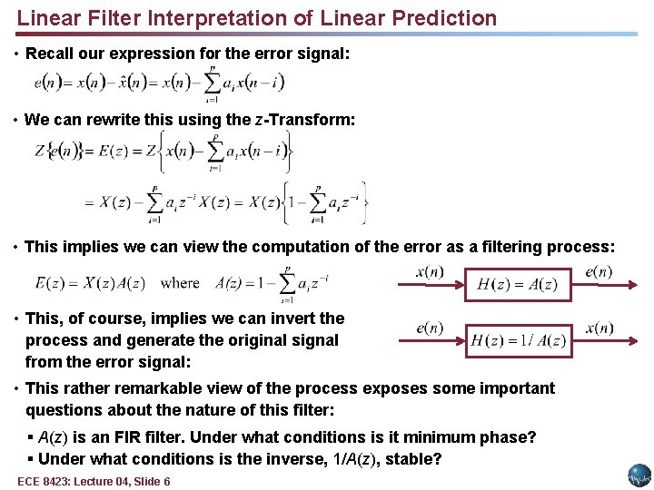
Linear Filter Interpretation of Linear Prediction • Recall our expression for the error signal: • We can rewrite this using the z-Transform: • This implies we can view the computation of the error as a filtering process: • This, of course, implies we can invert the process and generate the original signal from the error signal: • This rather remarkable view of the process exposes some important questions about the nature of this filter: § A(z) is an FIR filter. Under what conditions is it minimum phase? § Under what conditions is the inverse, 1/A(z), stable? ECE 8423: Lecture 04, Slide 6

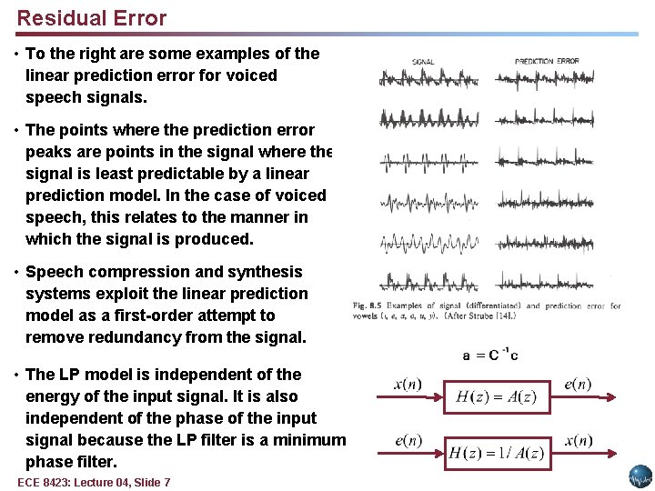
Residual Error • To the right are some examples of the linear prediction error for voiced speech signals. • The points where the prediction error peaks are points in the signal where the signal is least predictable by a linear prediction model. In the case of voiced speech, this relates to the manner in which the signal is produced. • Speech compression and synthesis systems exploit the linear prediction model as a first-order attempt to remove redundancy from the signal. • The LP model is independent of the energy of the input signal. It is also independent of the phase of the input signal because the LP filter is a minimum phase filter. ECE 8423: Lecture 04, Slide 7

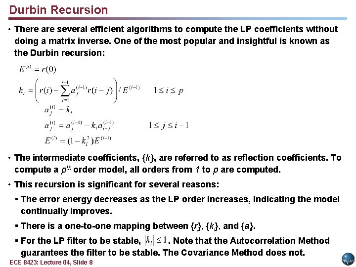
Durbin Recursion • There are several efficient algorithms to compute the LP coefficients without doing a matrix inverse. One of the most popular and insightful is known as the Durbin recursion: • The intermediate coefficients, {ki}, are referred to as reflection coefficients. To compute a pth order model, all orders from 1 to p are computed. • This recursion is significant for several reasons: § The error energy decreases as the LP order increases, indicating the model continually improves. § There is a one-to-one mapping between {ri}, {ki}, and {ai}. § For the LP filter to be stable, . Note that the Autocorrelation Method guarantees the filter to be stable. The Covariance Method does not. ECE 8423: Lecture 04, Slide 8

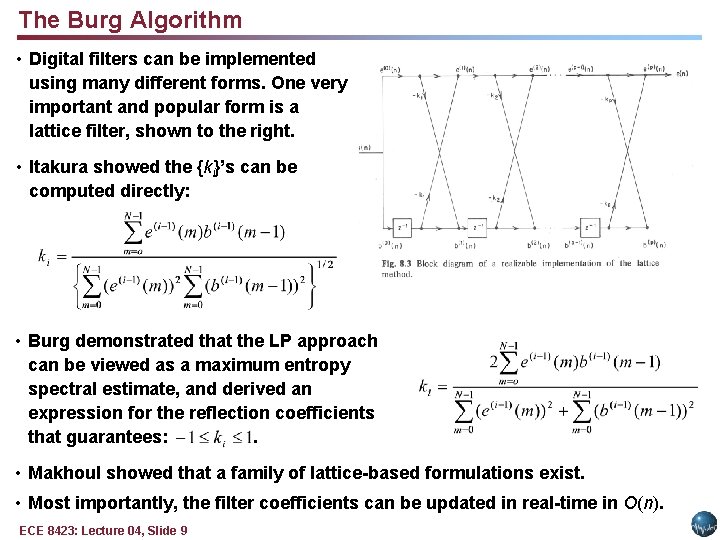
The Burg Algorithm • Digital filters can be implemented using many different forms. One very important and popular form is a lattice filter, shown to the right. • Itakura showed the {ki}’s can be computed directly: • Burg demonstrated that the LP approach can be viewed as a maximum entropy spectral estimate, and derived an expression for the reflection coefficients that guarantees: . • Makhoul showed that a family of lattice-based formulations exist. • Most importantly, the filter coefficients can be updated in real-time in O(n). ECE 8423: Lecture 04, Slide 9

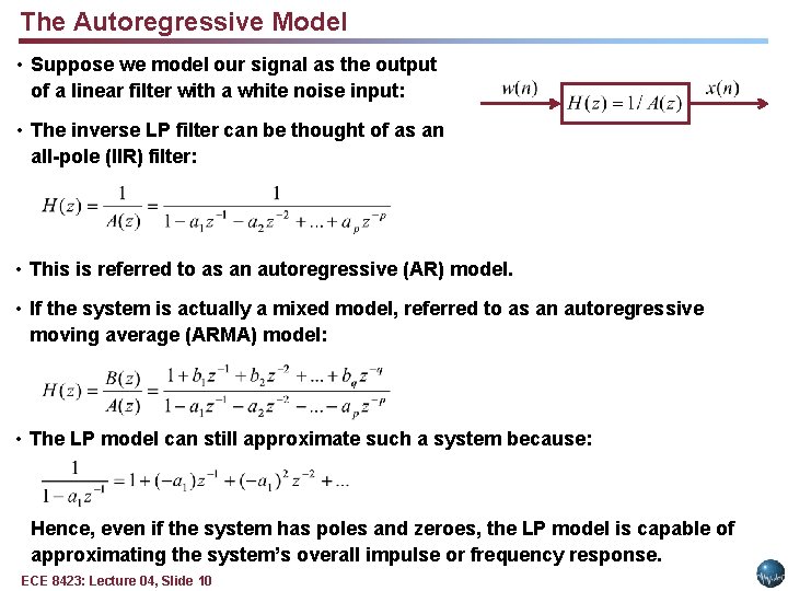
The Autoregressive Model • Suppose we model our signal as the output of a linear filter with a white noise input: • The inverse LP filter can be thought of as an all-pole (IIR) filter: • This is referred to as an autoregressive (AR) model. • If the system is actually a mixed model, referred to as an autoregressive moving average (ARMA) model: • The LP model can still approximate such a system because: Hence, even if the system has poles and zeroes, the LP model is capable of approximating the system’s overall impulse or frequency response. ECE 8423: Lecture 04, Slide 10

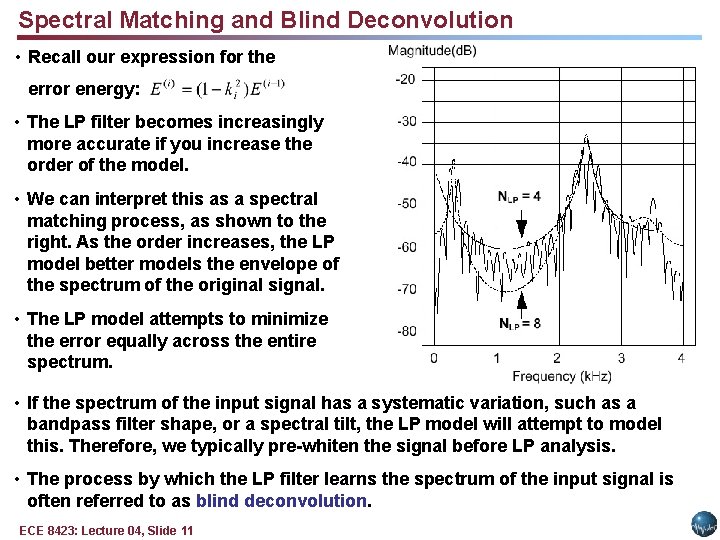
Spectral Matching and Blind Deconvolution • Recall our expression for the error energy: • The LP filter becomes increasingly more accurate if you increase the order of the model. • We can interpret this as a spectral matching process, as shown to the right. As the order increases, the LP model better models the envelope of the spectrum of the original signal. • The LP model attempts to minimize the error equally across the entire spectrum. • If the spectrum of the input signal has a systematic variation, such as a bandpass filter shape, or a spectral tilt, the LP model will attempt to model this. Therefore, we typically pre-whiten the signal before LP analysis. • The process by which the LP filter learns the spectrum of the input signal is often referred to as blind deconvolution. ECE 8423: Lecture 04, Slide 11

Summary • There are many interpretations and motivations for linear prediction ranging from minimum mean-square error estimation to maximum entropy spectral estimation. • There are many implementations of the filter, including the direct form and the lattice representation. • There are many representations for the coefficients including predictor and reflection coefficients. • The LP approach can be extended to estimate the parameters of most digital filters, and can also be applied to the problem of digital filter design. • The filter can be estimated in batch mode using a frame-based analysis, or it can be updated on a sample basis using a sequential or iterative estimator. Hence, the LP model is our first adaptive filter. Such a filter can be viewed as a time-varying digital filter that tracks a signal in real-time. • Under appropriate Gaussian assumptions, LP analysis can be shown to be a maximum likelihood estimate of the model parameters. • Further, two models can be compared using a metric called the log likelihood ratio. Many other metrics exist to compare such models, including cepstral and principal components approaches. ECE 8423: Lecture 04, Slide 12