ECE 6340 Intermediate EM Waves Fall 2016 Prof

ECE 6340 Intermediate EM Waves Fall 2016 Prof. David R. Jackson Dept. of ECE Notes 1 1

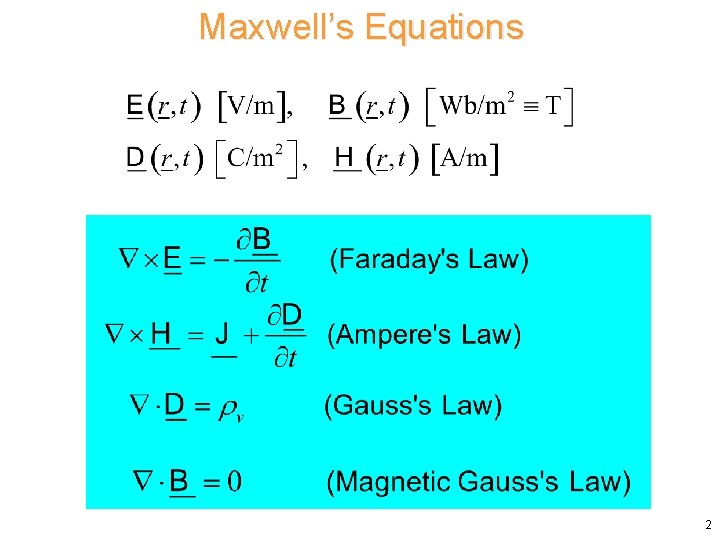
Maxwell’s Equations 2

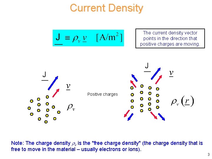
Current Density The current density vector points in the direction that positive charges are moving. Positive charges Note: The charge density v is the "free charge density" (the charge density that is free to move in the material – usually electrons or ions). 3

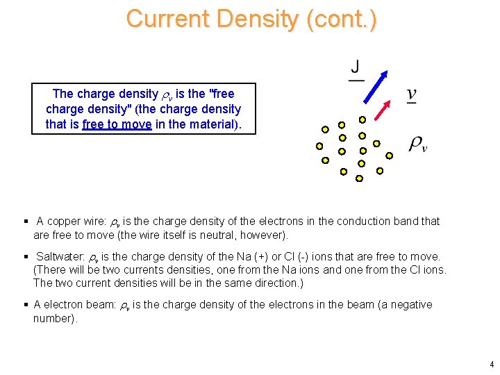
Current Density (cont. ) The charge density v is the "free charge density" (the charge density that is free to move in the material). § A copper wire: v is the charge density of the electrons in the conduction band that are free to move (the wire itself is neutral, however). § Saltwater: v is the charge density of the Na (+) or Cl (-) ions that are free to move. (There will be two currents densities, one from the Na ions and one from the Cl ions. The two current densities will be in the same direction. ) § A electron beam: v is the charge density of the electrons in the beam (a negative number). 4

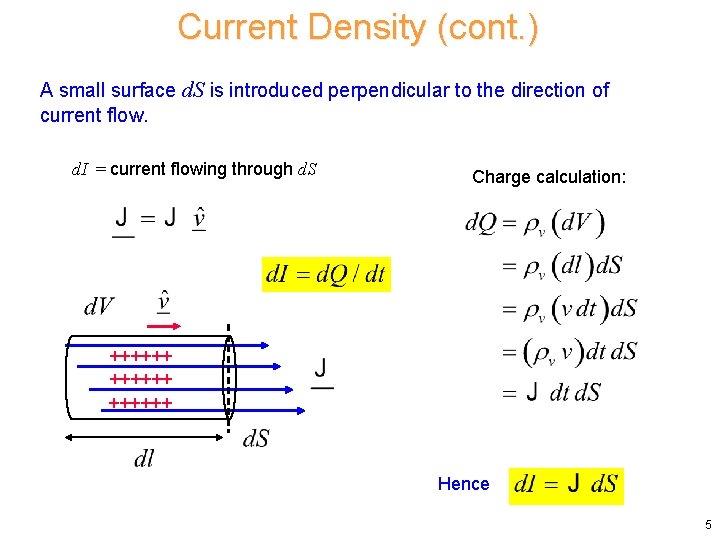
Current Density (cont. ) A small surface d. S is introduced perpendicular to the direction of current flow. d. I = current flowing through d. S Charge calculation: ++++++ Hence 5

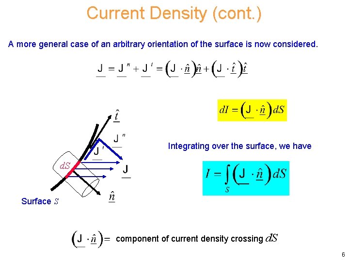
Current Density (cont. ) A more general case of an arbitrary orientation of the surface is now considered. Integrating over the surface, we have d. S Surface S component of current density crossing d. S 6

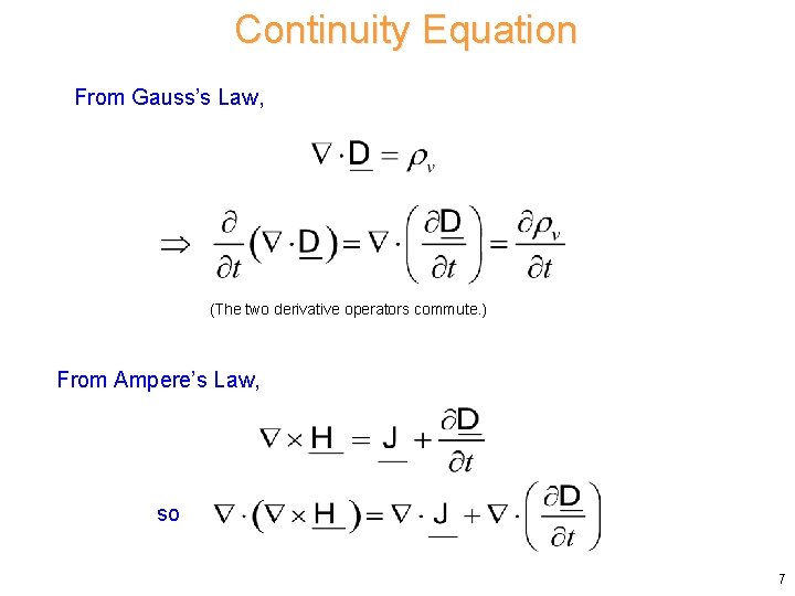
Continuity Equation From Gauss’s Law, (The two derivative operators commute. ) From Ampere’s Law, so 7

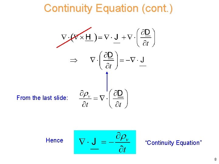
Continuity Equation (cont. ) From the last slide: Hence “Continuity Equation” 8

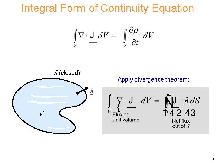
Integral Form of Continuity Equation S (closed) Apply divergence theorem: V 9

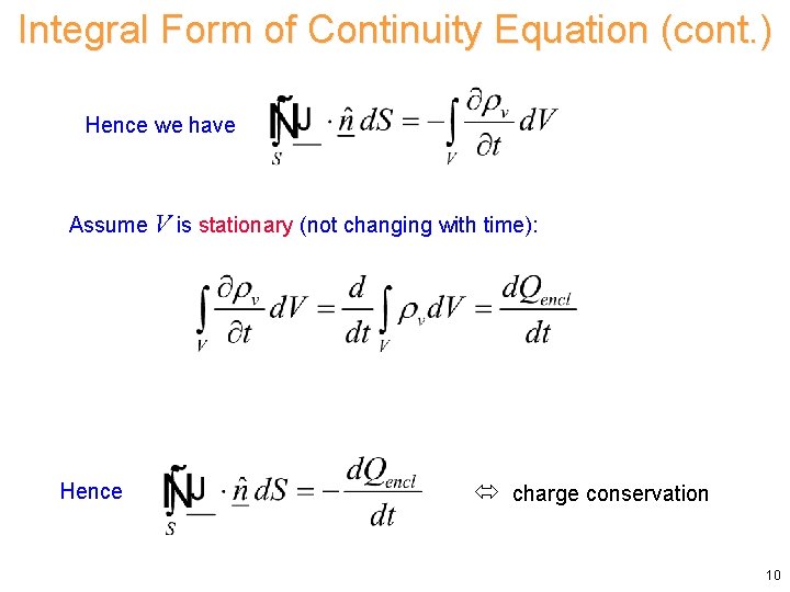
Integral Form of Continuity Equation (cont. ) Hence we have Assume V is stationary (not changing with time): Hence charge conservation 10

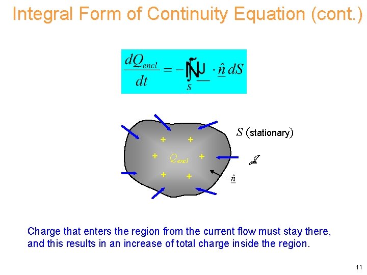
Integral Form of Continuity Equation (cont. ) + + + Qencl + S (stationary) + J + Charge that enters the region from the current flow must stay there, and this results in an increase of total charge inside the region. 11

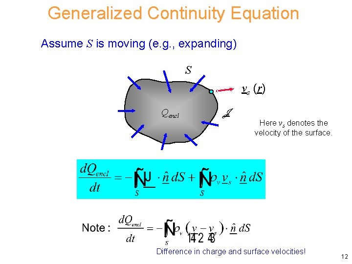
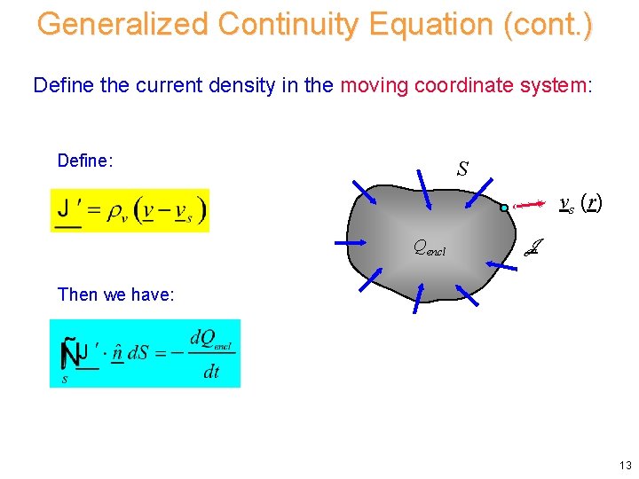
Generalized Continuity Equation Assume S is moving (e. g. , expanding) S vs (r) Qencl J Here vs denotes the velocity of the surface. Difference in charge and surface velocities! 12

Generalized Continuity Equation (cont. ) Define the current density in the moving coordinate system: Define: S vs (r) Qencl J Then we have: 13

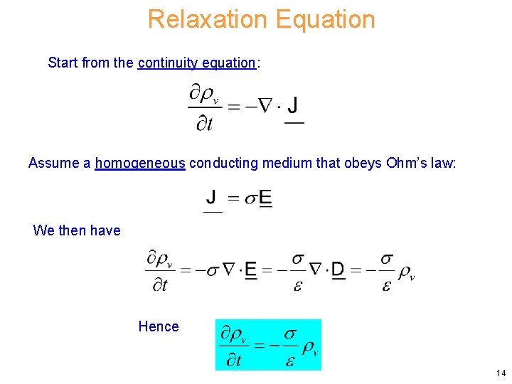
Relaxation Equation Start from the continuity equation: Assume a homogeneous conducting medium that obeys Ohm’s law: We then have Hence 14

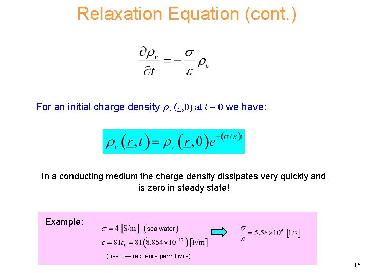
Relaxation Equation (cont. ) For an initial charge density v (r, 0) at t = 0 we have: In a conducting medium the charge density dissipates very quickly and is zero in steady state! Example: (use low-frequency permittivity) 15

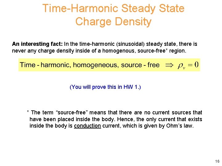
Time-Harmonic Steady State Charge Density An interesting fact: In the time-harmonic (sinusoidal) steady state, there is never any charge density inside of a homogenous, source-free* region. (You will prove this in HW 1. ) * The term “source-free” means that there are no current sources that have been placed inside the body. Hence, the only current that exists inside the body is conduction current, which is given by Ohm’s law. 16

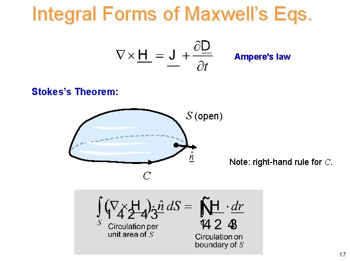
Integral Forms of Maxwell’s Eqs. Ampere's law Stokes’s Theorem: S (open) Note: right-hand rule for C. C 17

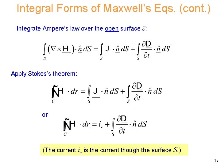
Integral Forms of Maxwell’s Eqs. (cont. ) Integrate Ampere’s law over the open surface S: Apply Stokes’s theorem: or (The current is is the current though the surface S. ) 18

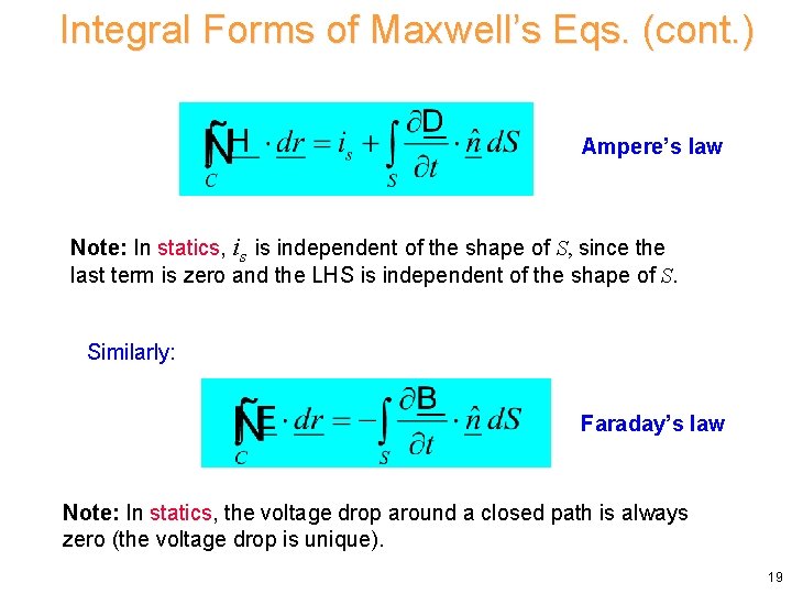
Integral Forms of Maxwell’s Eqs. (cont. ) Ampere’s law Note: In statics, is is independent of the shape of S, since the last term is zero and the LHS is independent of the shape of S. Similarly: Faraday’s law Note: In statics, the voltage drop around a closed path is always zero (the voltage drop is unique). 19

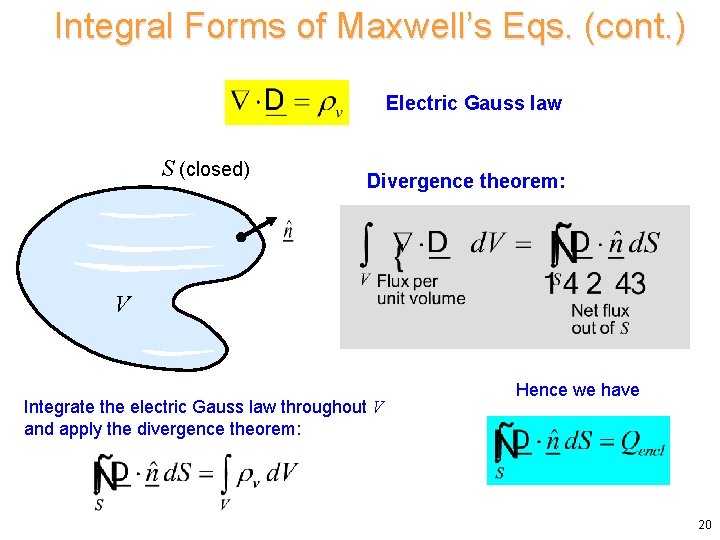
Integral Forms of Maxwell’s Eqs. (cont. ) Electric Gauss law S (closed) Divergence theorem: V Integrate the electric Gauss law throughout V and apply the divergence theorem: Hence we have 20

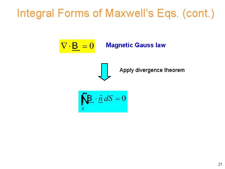
Integral Forms of Maxwell’s Eqs. (cont. ) Magnetic Gauss law Apply divergence theorem 21

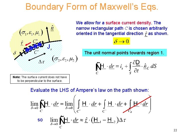
Boundary Form of Maxwell’s Eqs. We allow for a surface current density. The narrow rectangular path C is chosen arbitrarily oriented in the tangential direction as shown. The unit normal points towards region 1. Note: The surface current does not have to be perpendicular to the surface. Evaluate the LHS of Ampere’s law on the path shown: so 22

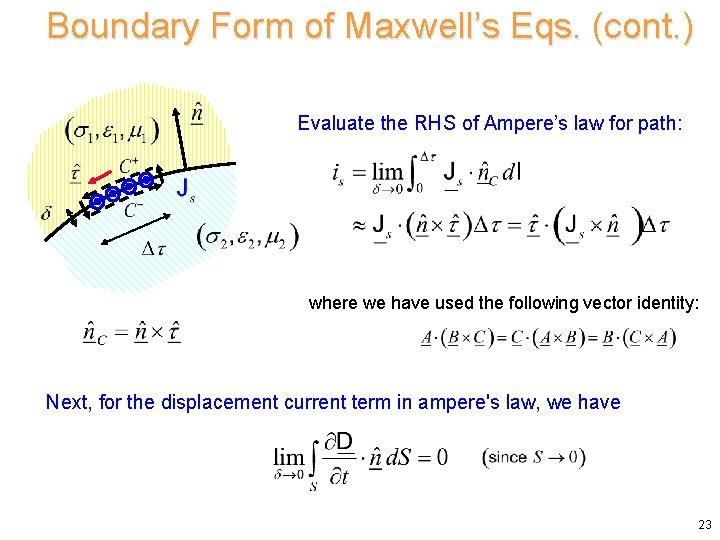
Boundary Form of Maxwell’s Eqs. (cont. ) Evaluate the RHS of Ampere’s law for path: where we have used the following vector identity: Next, for the displacement current term in ampere's law, we have 23

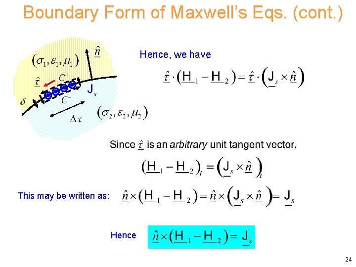
Boundary Form of Maxwell’s Eqs. (cont. ) Hence, we have This may be written as: Hence 24

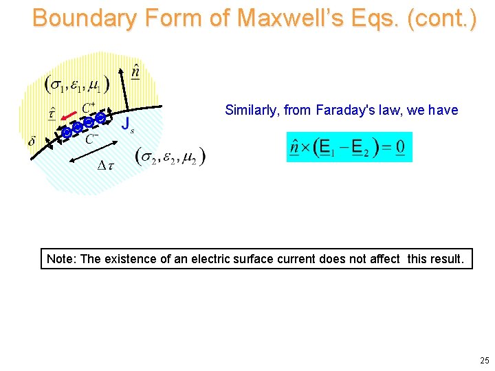
Boundary Form of Maxwell’s Eqs. (cont. ) Similarly, from Faraday's law, we have Note: The existence of an electric surface current does not affect this result. 25

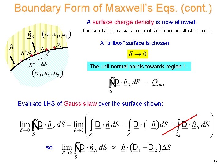
Boundary Form of Maxwell’s Eqs. (cont. ) A surface charge density is now allowed. There could also be a surface current, but it does not affect the result. + + + A “pillbox” surface is chosen. The unit normal points towards region 1. Evaluate LHS of Gauss’s law over the surface shown: so 26

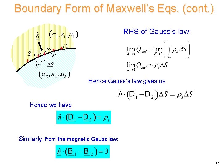
Boundary Form of Maxwell’s Eqs. (cont. ) RHS of Gauss’s law: + + + Hence Gauss’s law gives us Hence we have Similarly, from the magnetic Gauss law: 27

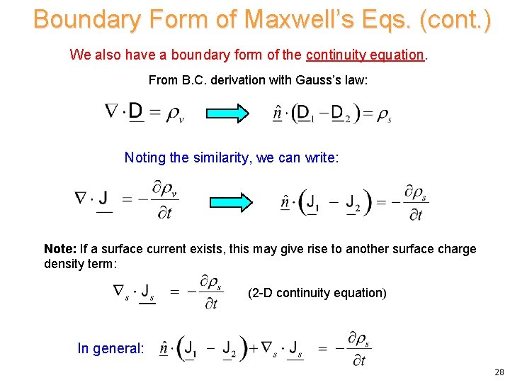
Boundary Form of Maxwell’s Eqs. (cont. ) We also have a boundary form of the continuity equation. From B. C. derivation with Gauss’s law: Noting the similarity, we can write: Note: If a surface current exists, this may give rise to another surface charge density term: (2 -D continuity equation) In general: 28

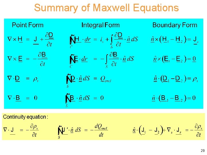
Summary of Maxwell Equations 29

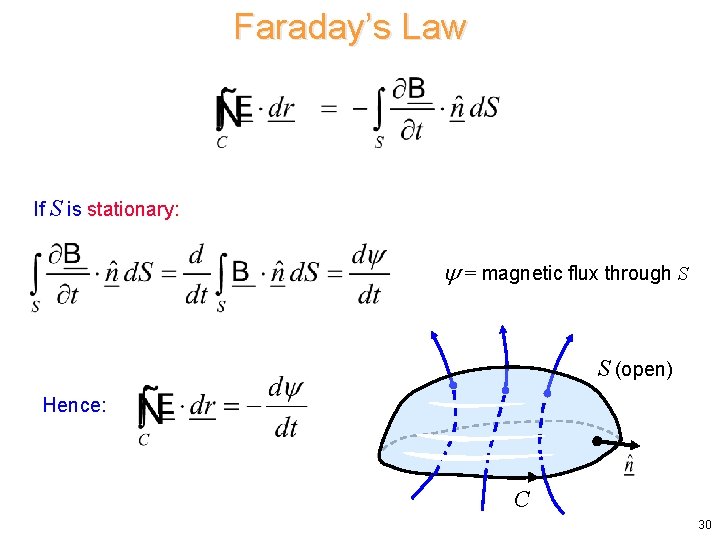
Faraday’s Law If S is stationary: = magnetic flux through S S (open) Hence: C 30

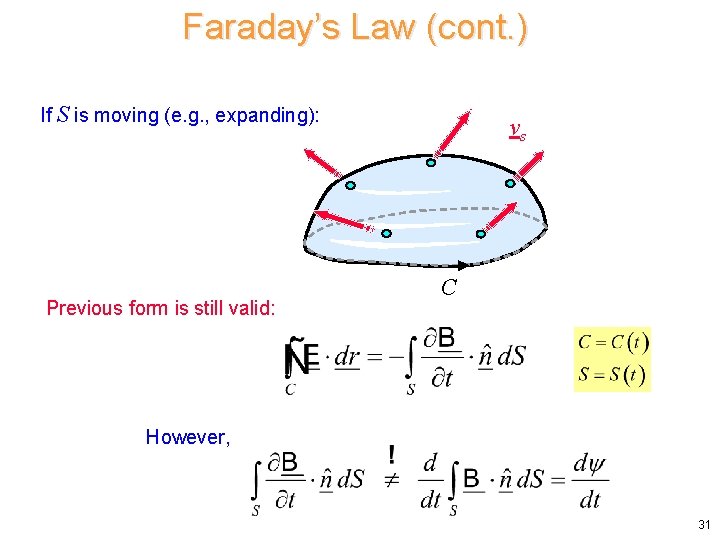
Faraday’s Law (cont. ) If S is moving (e. g. , expanding): Previous form is still valid: vs C However, 31

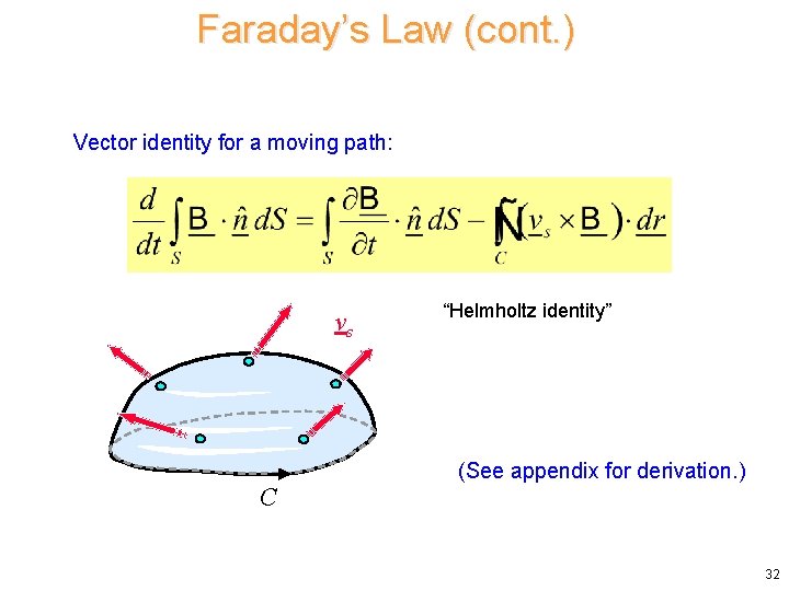
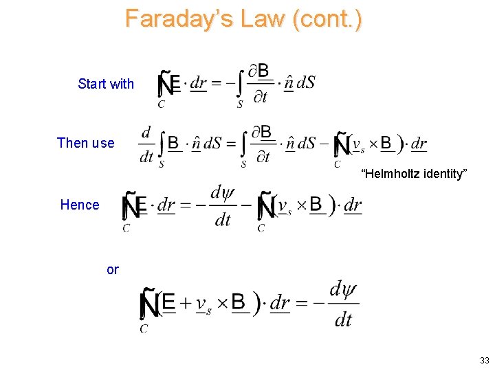
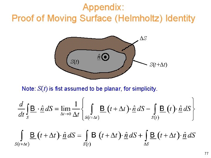
Faraday’s Law (cont. ) Vector identity for a moving path: vs C “Helmholtz identity” (See appendix for derivation. ) 32

Faraday’s Law (cont. ) Start with Then use “Helmholtz identity” Hence or 33

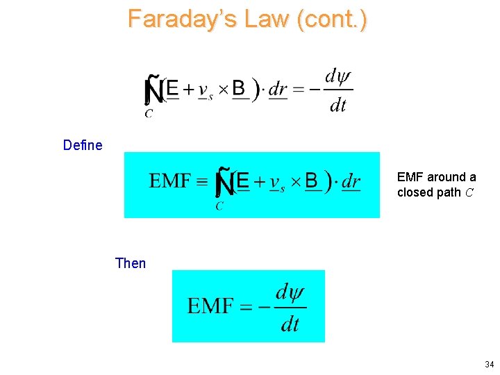
Faraday’s Law (cont. ) Define EMF around a closed path C Then 34

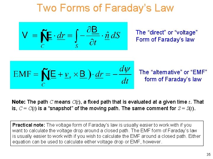
Two Forms of Faraday’s Law The “direct” or “voltage” Form of Faraday’s law The “alternative” or “EMF” form of Faraday’s law Note: The path C means C(t), a fixed path that is evaluated at a given time t. That is, C = C(t) is a “snapshot” of the moving path. The same comment for S = S(t). Practical note: The voltage form of Faraday’s law is usually easier to work with if you want to calculate the voltage drop around a closed path. The EMF form of Faraday’s law is usually easier to work with if you wish to calculate the EMF around a closed path. Either equation can be used to calculate either voltage drop or EMF, however. 35

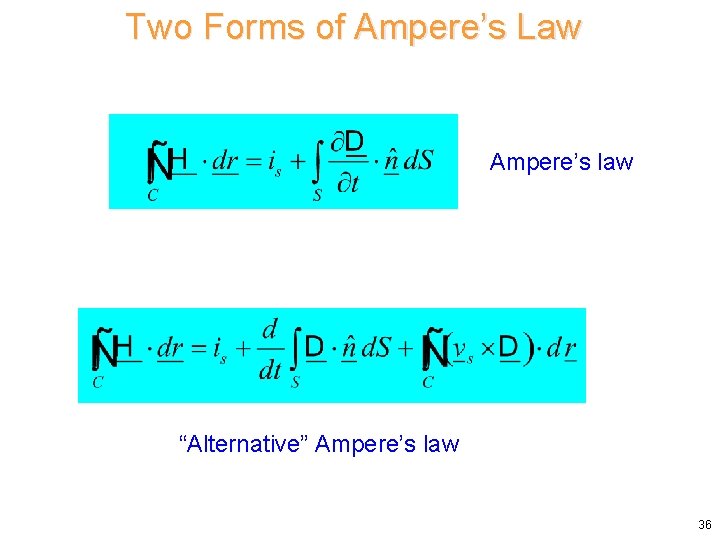
Two Forms of Ampere’s Law Ampere’s law “Alternative” Ampere’s law 36

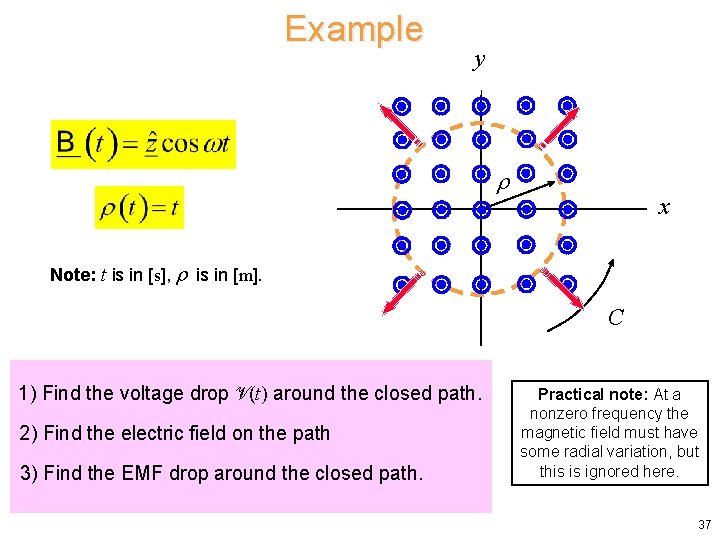
Example y x Note: t is in [s], is in [m]. C 1) Find the voltage drop V(t) around the closed path. 2) Find the electric field on the path 3) Find the EMF drop around the closed path. Practical note: At a nonzero frequency the magnetic field must have some radial variation, but this is ignored here. 37

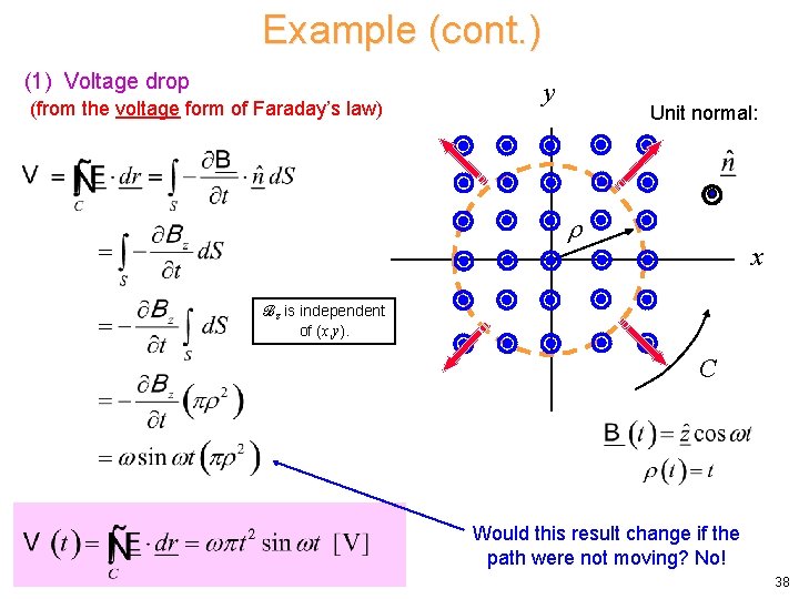
Example (cont. ) (1) Voltage drop (from the voltage form of Faraday’s law) y Unit normal: x Bz is independent of (x, y). C Would this result change if the path were not moving? No! 38

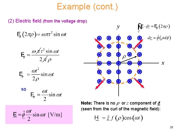
Example (cont. ) (2) Electric field (from the voltage drop) y x so Note: There is no or z component of E (seen from the curl of the magnetic field): 39

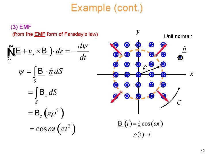
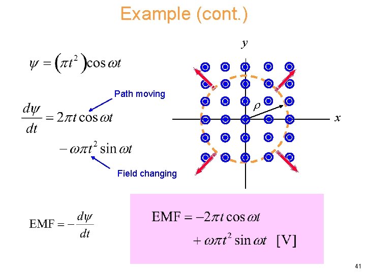
Example (cont. ) (3) EMF (from the EMF form of Faraday’s law) y Unit normal: x C 40

Example (cont. ) y Path moving x Field changing 41

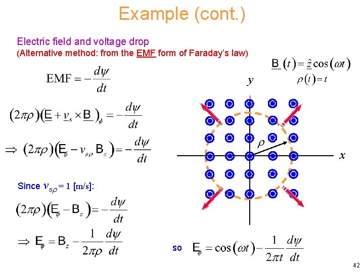
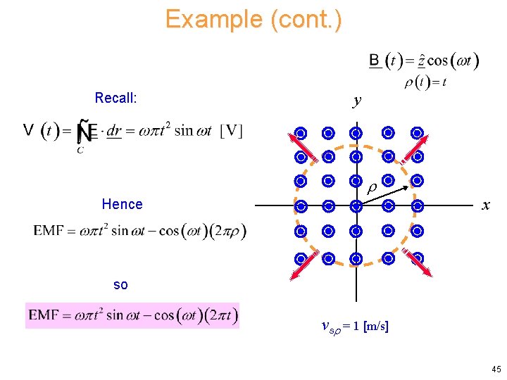
Example (cont. ) Electric field and voltage drop (Alternative method: from the EMF form of Faraday’s law) y x Since vs = 1 [m/s]: so 42

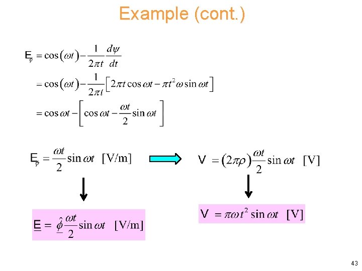
Example (cont. ) 43

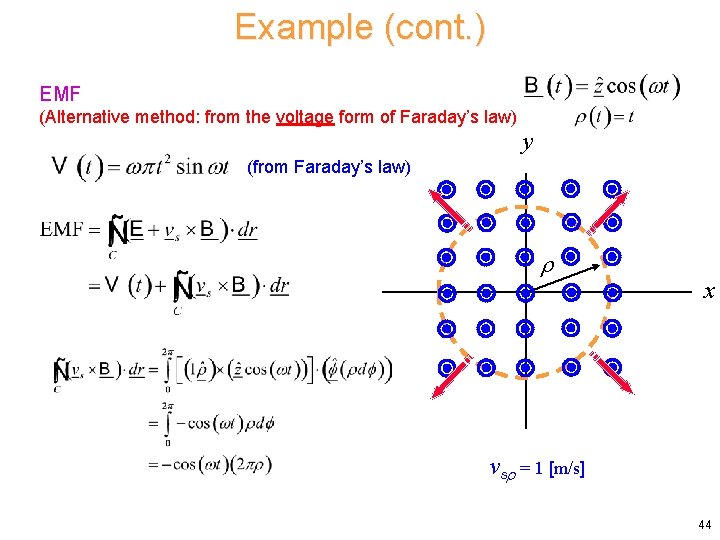
Example (cont. ) EMF (Alternative method: from the voltage form of Faraday’s law) y (from Faraday’s law) x vs = 1 [m/s] 44

Example (cont. ) Recall: y Hence x so vs = 1 [m/s] 45

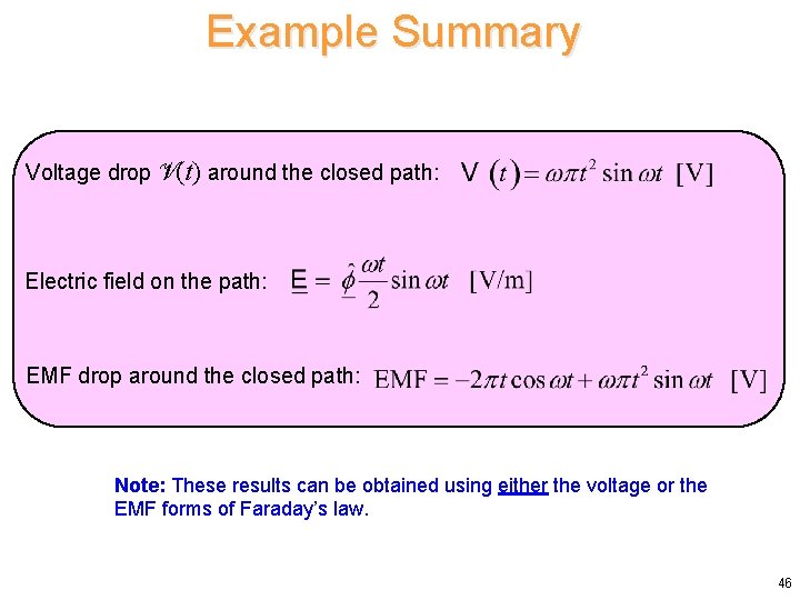
Example Summary Voltage drop V(t) around the closed path: Electric field on the path: EMF drop around the closed path: Note: These results can be obtained using either the voltage or the EMF forms of Faraday’s law. 46

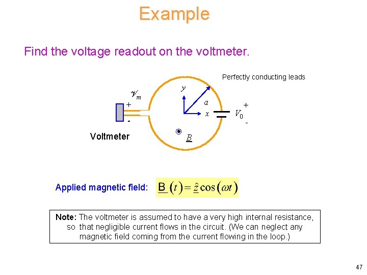
Example Find the voltage readout on the voltmeter. Perfectly conducting leads Vm + y a x Voltmeter V 0 + - B Applied magnetic field: Note: The voltmeter is assumed to have a very high internal resistance, so that negligible current flows in the circuit. (We can neglect any magnetic field coming from the current flowing in the loop. ) 47

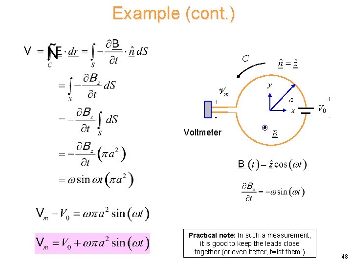
Example (cont. ) C Vm + y a x Voltmeter V 0 + - B Practical note: In such a measurement, it is good to keep the leads close together (or even better, twist them. ) 48

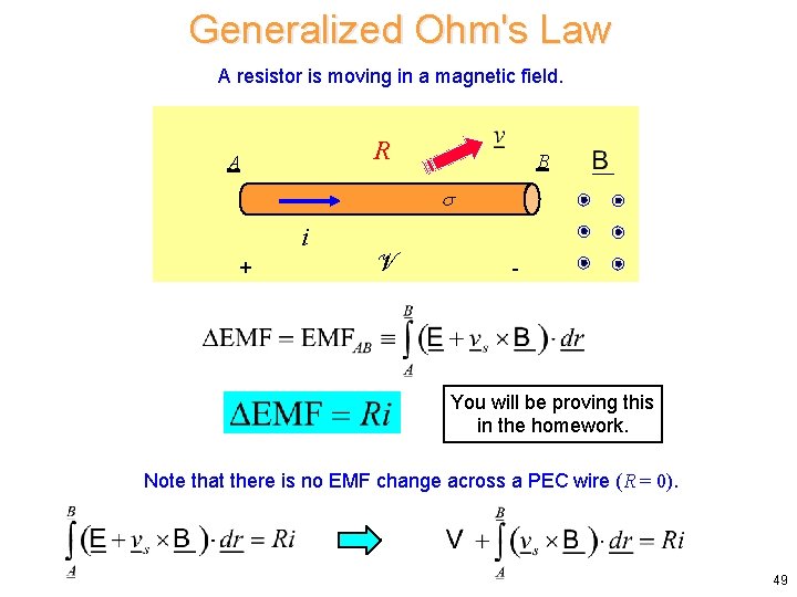
Generalized Ohm's Law A resistor is moving in a magnetic field. R A B i + V - You will be proving this in the homework. Note that there is no EMF change across a PEC wire (R = 0). 49

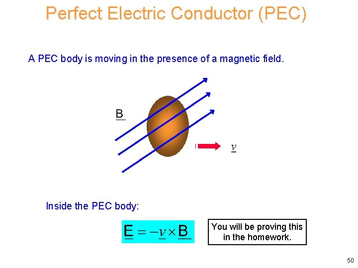
Perfect Electric Conductor (PEC) A PEC body is moving in the presence of a magnetic field. Inside the PEC body: You will be proving this in the homework. 50

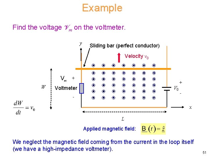
Example Find the voltage Vm on the voltmeter. y Sliding bar (perfect conductor) Velocity v 0 + W V 0 Voltmeter - + - x L Applied magnetic field: We neglect the magnetic field coming from the current in the loop itself (we have a high-impedance voltmeter). 51

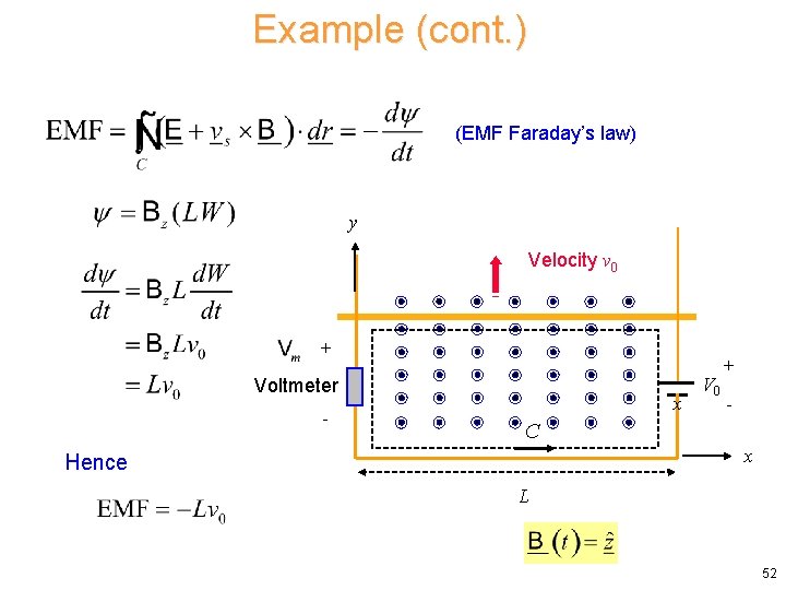
Example (cont. ) (EMF Faraday’s law) y Velocity v 0 + Voltmeter - x V 0 + - C x Hence L 52

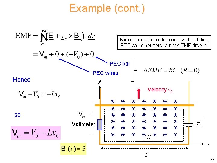
Example (cont. ) Note: The voltage drop across the sliding PEC bar is not zero, but the EMF drop is. PEC bar PEC wires y Hence Velocity v 0 so + V 0 Voltmeter - + - C x L 53

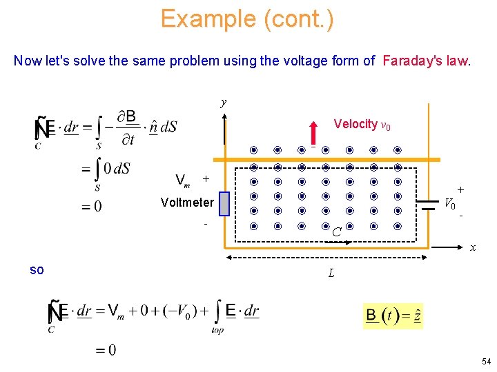
Example (cont. ) Now let's solve the same problem using the voltage form of Faraday's law. y Velocity v 0 + V 0 Voltmeter - + - C x so L 54

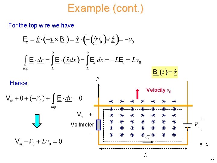
Example (cont. ) For the top wire we have y Hence Velocity v 0 + Voltmeter - x V 0 + - C x L 55

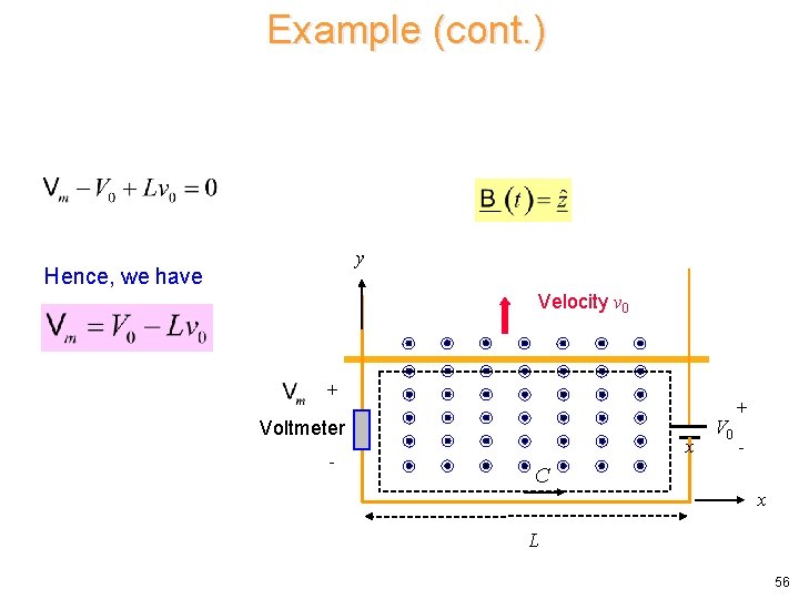
Example (cont. ) y Hence, we have Velocity v 0 + Voltmeter - x V 0 + - C x L 56

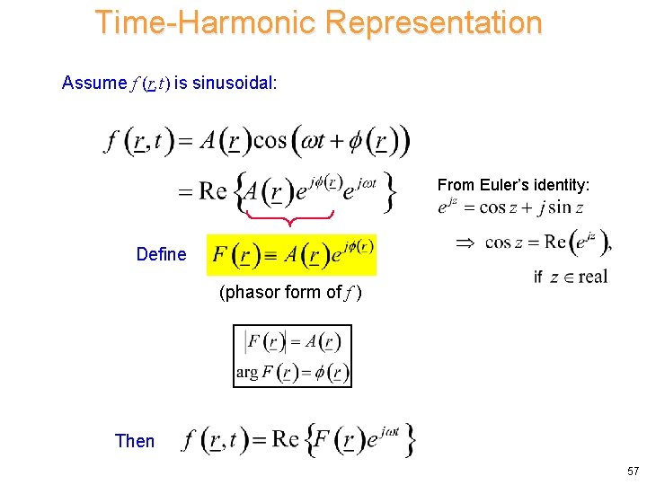
Time-Harmonic Representation Assume f (r, t) is sinusoidal: From Euler’s identity: Define (phasor form of f ) Then 57

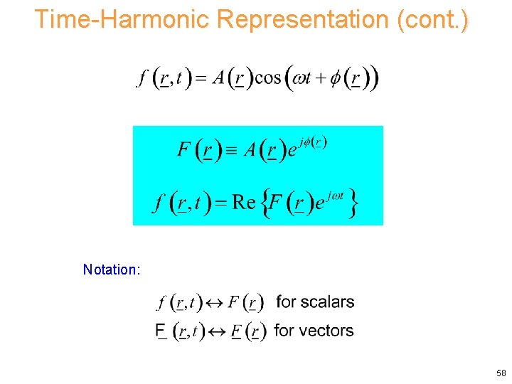
Time-Harmonic Representation (cont. ) Notation: 58

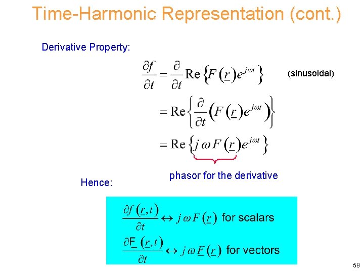
Time-Harmonic Representation (cont. ) Derivative Property: (sinusoidal) Hence: phasor for the derivative 59

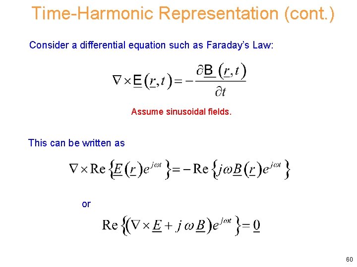
Time-Harmonic Representation (cont. ) Consider a differential equation such as Faraday’s Law: Assume sinusoidal fields. This can be written as or 60

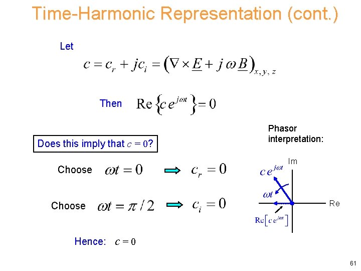
Time-Harmonic Representation (cont. ) Let Then Does this imply that c = 0? Im Choose Re Choose Hence: Phasor interpretation: c=0 61

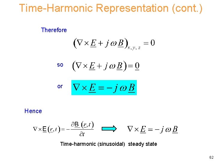
Time-Harmonic Representation (cont. ) Therefore so or Hence Time-harmonic (sinusoidal) steady state 62

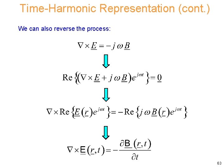
Time-Harmonic Representation (cont. ) We can also reverse the process: 63

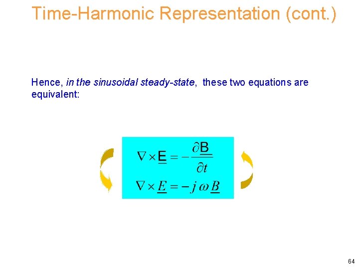
Time-Harmonic Representation (cont. ) Hence, in the sinusoidal steady-state, these two equations are equivalent: 64

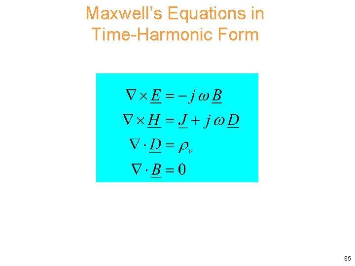
Maxwell’s Equations in Time-Harmonic Form 65

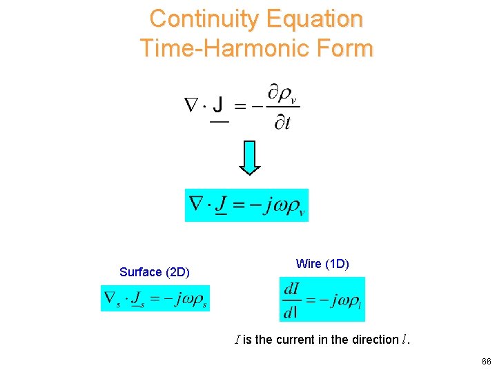
Continuity Equation Time-Harmonic Form Surface (2 D) Wire (1 D) I is the current in the direction l. 66

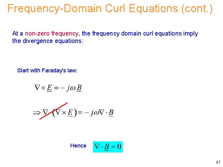
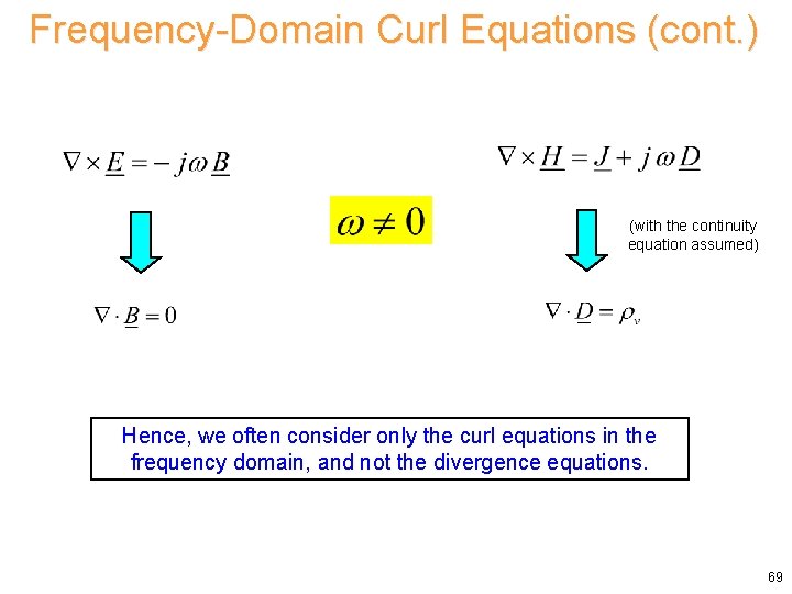
Frequency-Domain Curl Equations (cont. ) At a non-zero frequency, the frequency domain curl equations imply the divergence equations: Start with Faraday's law: Hence 67

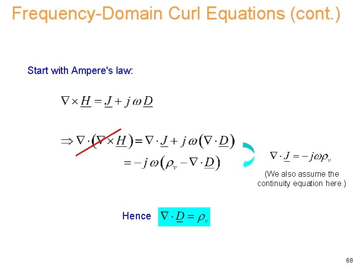
Frequency-Domain Curl Equations (cont. ) Start with Ampere's law: (We also assume the continuity equation here. ) Hence 68

Frequency-Domain Curl Equations (cont. ) (with the continuity equation assumed) Hence, we often consider only the curl equations in the frequency domain, and not the divergence equations. 69

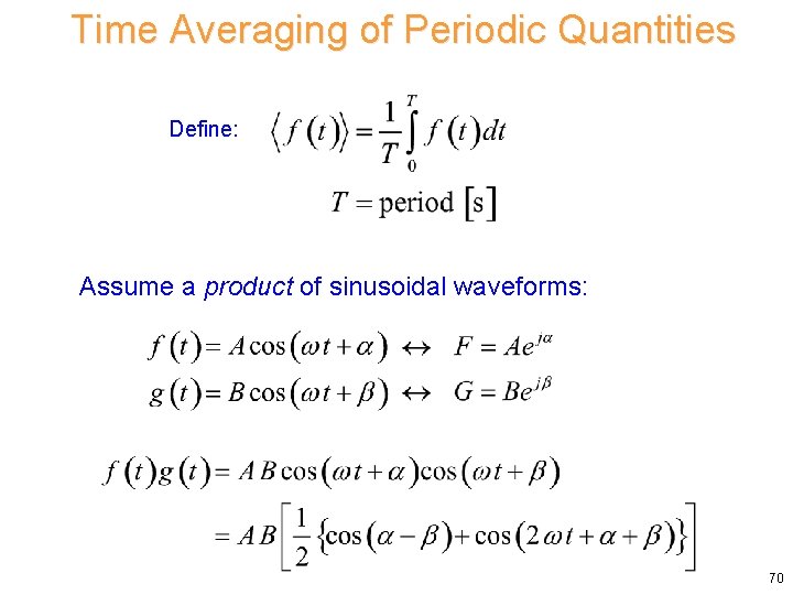
Time Averaging of Periodic Quantities Define: Assume a product of sinusoidal waveforms: 70

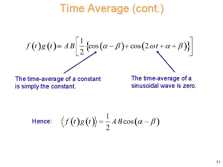
Time Average (cont. ) The time-average of a constant is simply the constant. The time-average of a sinusoidal wave is zero. Hence: 71

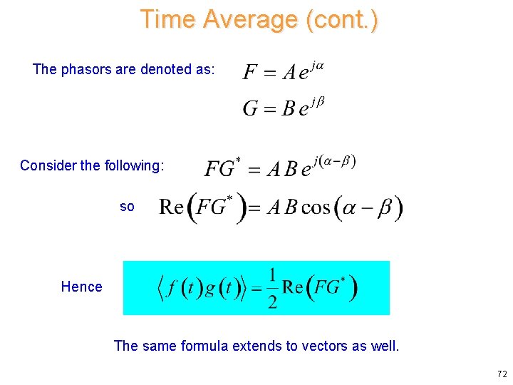
Time Average (cont. ) The phasors are denoted as: Consider the following: so Hence The same formula extends to vectors as well. 72

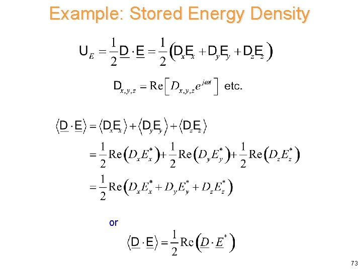
Example: Stored Energy Density or 73

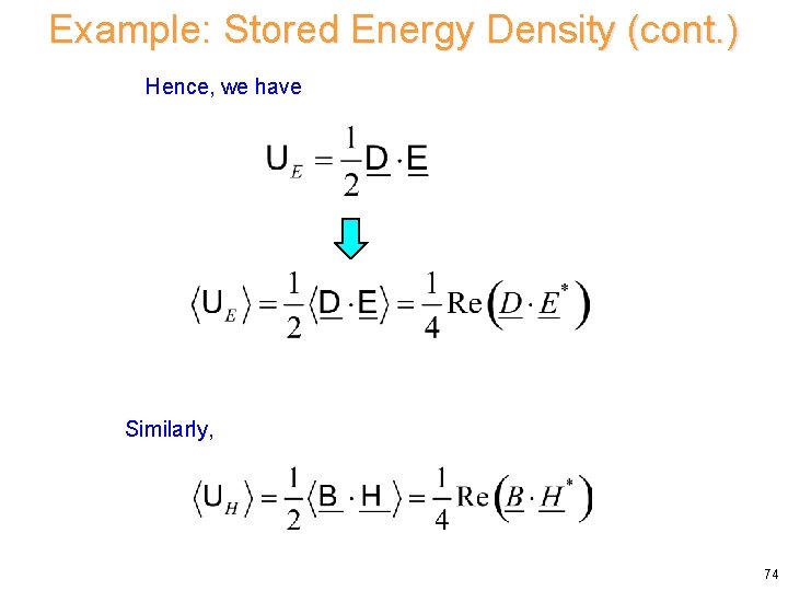
Example: Stored Energy Density (cont. ) Hence, we have Similarly, 74

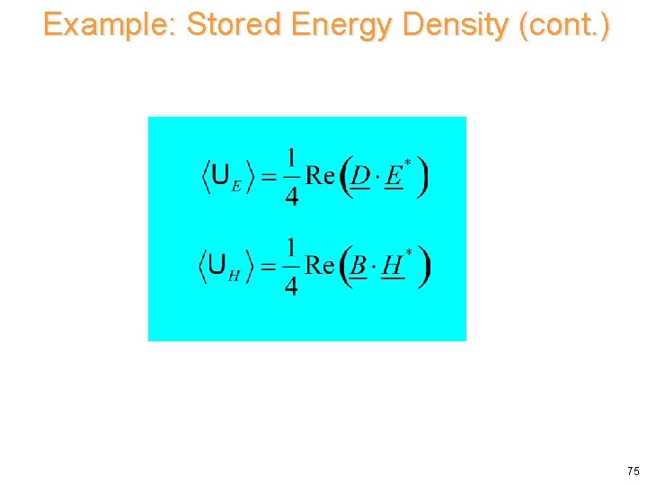
Example: Stored Energy Density (cont. ) 75

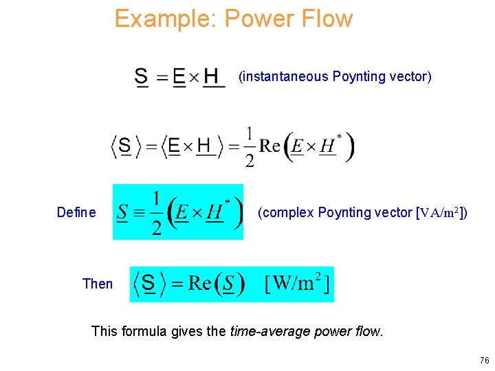
Example: Power Flow (instantaneous Poynting vector) Define (complex Poynting vector [VA/m 2]) Then This formula gives the time-average power flow. 76

Appendix: Proof of Moving Surface (Helmholtz) Identity S S(t) S(t+ t) Note: S(t) is fist assumed to be planar, for simplicity. 77

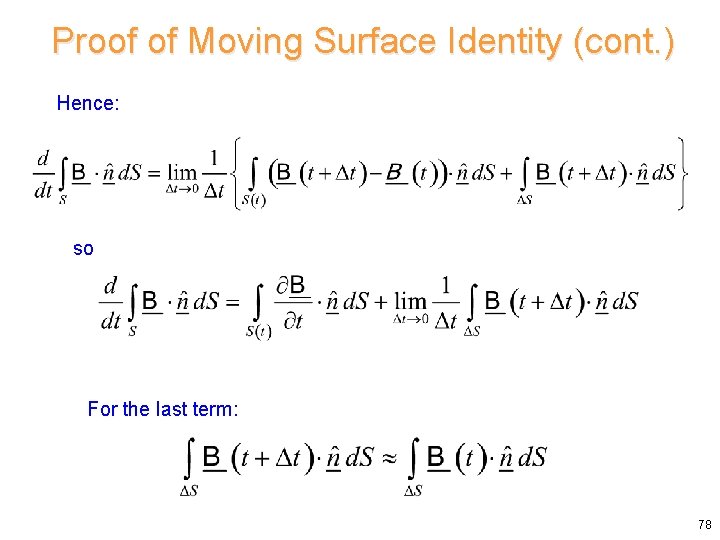
Proof of Moving Surface Identity (cont. ) Hence: so For the last term: 78

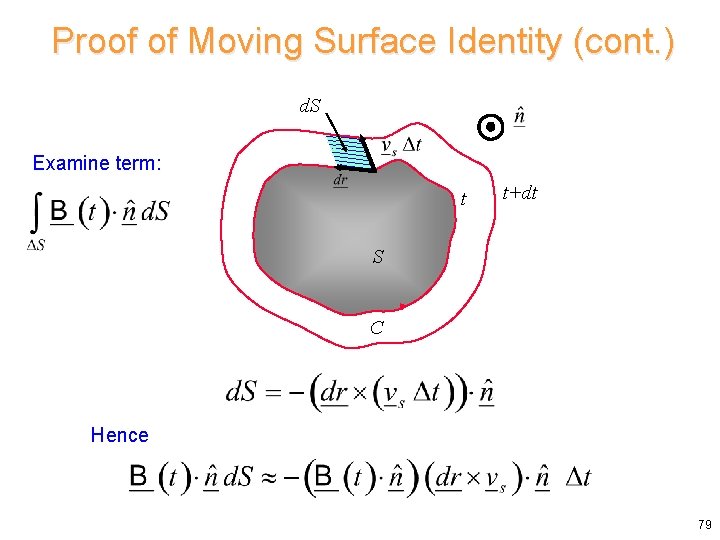
Proof of Moving Surface Identity (cont. ) d. S Examine term: t t+dt S C Hence 79

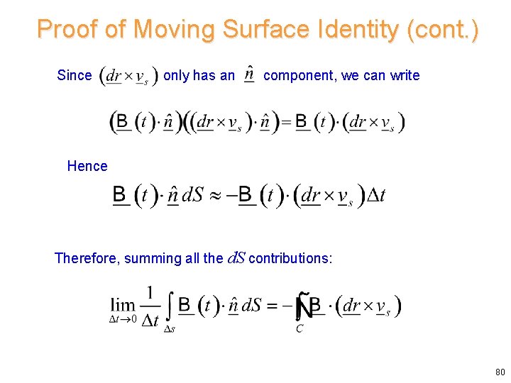
Proof of Moving Surface Identity (cont. ) Since only has an component, we can write Hence Therefore, summing all the d. S contributions: 80

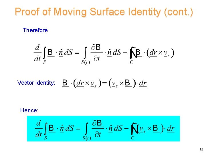
Proof of Moving Surface Identity (cont. ) Therefore Vector identity: Hence: 81

Proof of Moving Surface Identity (cont. ) Notes: § If the surface S is non-planar, the result still holds, since the magnetic flux through any two surfaces that end on C must be the same, since the divergence of the magnetic field is zero (from the magnetic Gauss law). Hence, the surface can always be chosen as planar for the purposes of calculating the magnetic flux through the surface. § The identity can also be extended to the case where the contour C is nonplanar, but the proof is omitted here. 82