ECE 576 POWER SYSTEM DYNAMICS AND STABILITY Lecture

ECE 576 POWER SYSTEM DYNAMICS AND STABILITY Lecture 24 Initial conditions Professor M. A. Pai Department of Electrical and Computer Engineering © 2000 University of Illinois Board of Trustees, All Rights Reserved

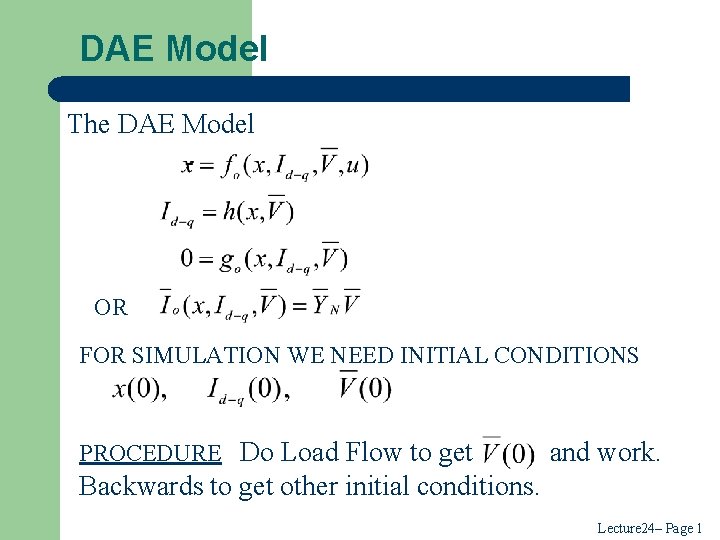
DAE Model The DAE Model OR FOR SIMULATION WE NEED INITIAL CONDITIONS PROCEDURE Do Load Flow to get and work. Backwards to get other initial conditions. Lecture 24– Page 1

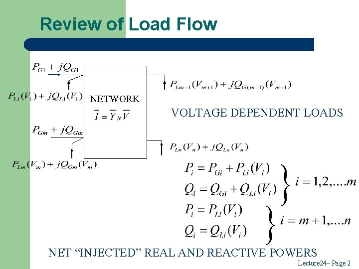
Review of Load Flow NETWORK VOLTAGE DEPENDENT LOADS NET “INJECTED” REAL AND REACTIVE POWERS Lecture 24– Page 2

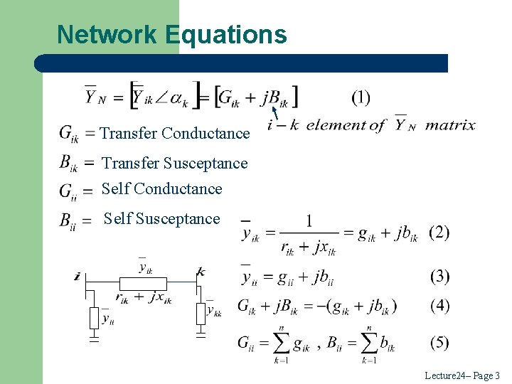
Network Equations Transfer Conductance Transfer Susceptance Self Conductance Self Susceptance Lecture 24– Page 3

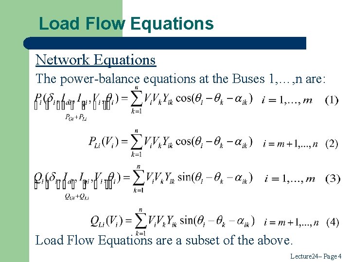
Load Flow Equations Network Equations The power-balance equations at the Buses 1, …, n are: Load Flow Equations are a subset of the above. Lecture 24– Page 4

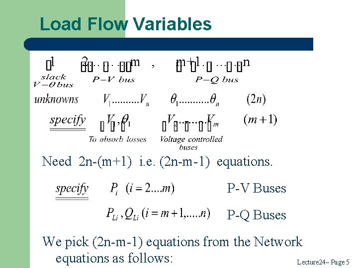
Load Flow Variables 1 2………m , m+1………n Need 2 n-(m+1) i. e. (2 n-m-1) equations. P-V Buses P-Q Buses We pick (2 n-m-1) equations from the Network equations as follows: Lecture 24– Page 5

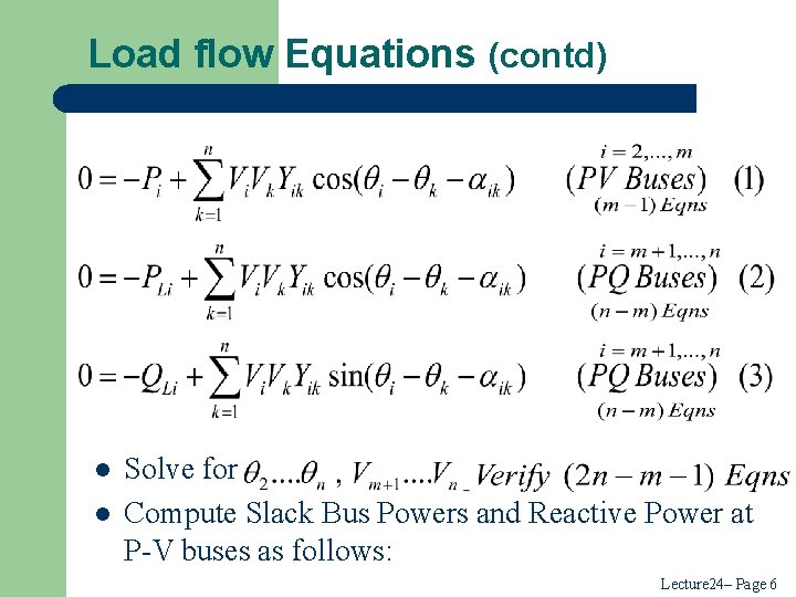
Load flow Equations (contd) l l Solve for Compute Slack Bus Powers and Reactive Power at P-V buses as follows: Lecture 24– Page 6

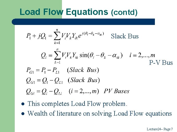
Load Flow Equations (contd) Slack Bus P-V Bus l l This completes Load Flow problem. Wealth of literature on solving Load Flow equations Lecture 24– Page 7

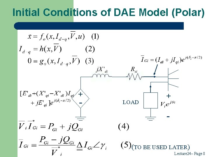
Initial Conditions of DAE Model (Polar) + - LOAD + (TO BE USED LATER) Lecture 24– Page 8

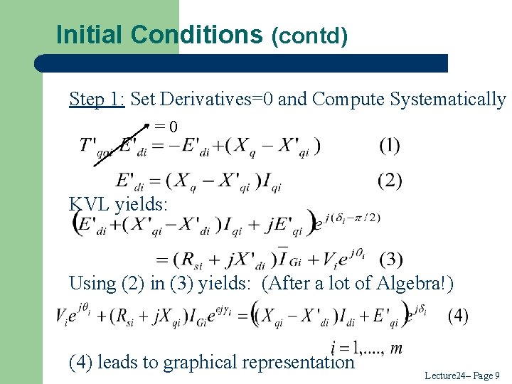
Initial Conditions (contd) Step 1: Set Derivatives=0 and Compute Systematically =0 KVL yields: Using (2) in (3) yields: (After a lot of Algebra!) (4) leads to graphical representation Lecture 24– Page 9

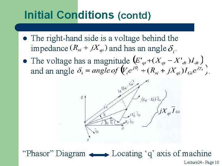
Initial Conditions (contd) l l The right-hand side is a voltage behind the impedance and has an angle. The voltage has a magnitude and an angle “Phasor” Diagram . Locating ‘q’ axis of machine Lecture 24– Page 10

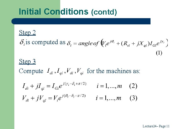
Initial Conditions (contd) Step 2 is computed as Step 3 Compute for the machines as: Lecture 24– Page 11

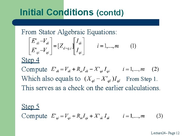
Initial Conditions (contd) From Stator Algebraic Equations: Step 4 Compute Which also equals to From Step 1. This serves as a check on the earlier calculations. Step 5 Compute Lecture 24– Page 12

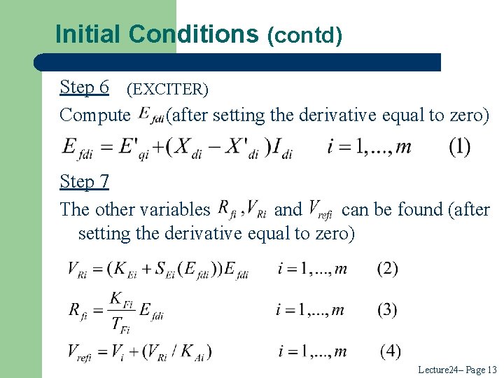
Initial Conditions (contd) Step 6 (EXCITER) Compute (after setting the derivative equal to zero) Step 7 The other variables and can be found (after setting the derivative equal to zero) Lecture 24– Page 13

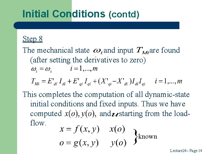
Initial Conditions (contd) Step 8 The mechanical state and input are found (after setting the derivatives to zero) This completes the computation of all dynamic-state initial conditions and fixed inputs. Thus we have computed and starting from the loadflow. } known Lecture 24– Page 14

Initial Conditions (contd) l l For a given disturbance, the inputs remain fixed throughout the simulation. If the disturbance occurs due to a fault or a network change, the algebraic states must change instantaneously. Dynamic states cannot change instantaneously. Hence solve all the algebraic equations inclusive of the stator equations with the dynamic states specified at their values just prior to the disturbance as initial conditions to determine the new initial values of the algebraic states. Lecture 24– Page 15

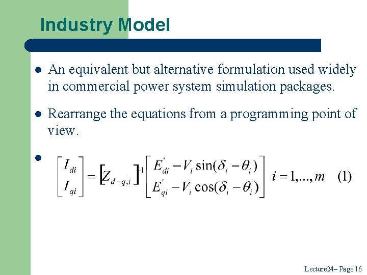
Industry Model l An equivalent but alternative formulation used widely in commercial power system simulation packages. l Rearrange the equations from a programming point of view. l . Lecture 24– Page 16

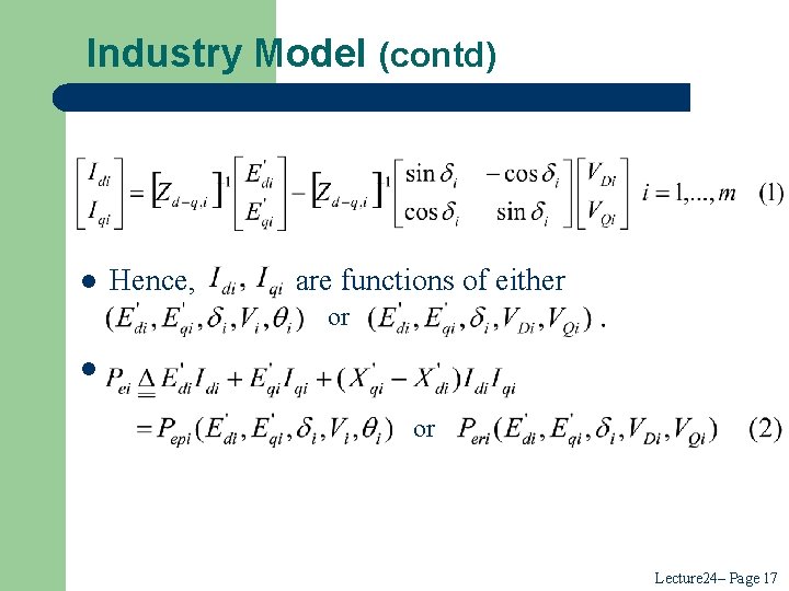
Industry Model (contd) l Hence, are functions of either or l . or Lecture 24– Page 17

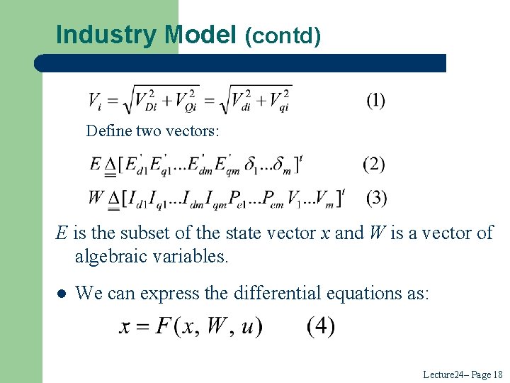
Industry Model (contd) Define two vectors: E is the subset of the state vector x and W is a vector of algebraic variables. l We can express the differential equations as: Lecture 24– Page 18

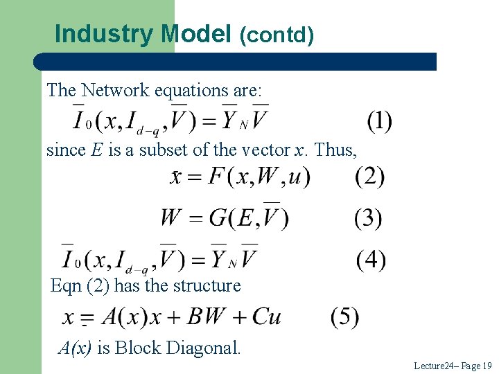
Industry Model (contd) The Network equations are: since E is a subset of the vector x. Thus, Eqn (2) has the structure A(x) is Block Diagonal. Lecture 24– Page 19

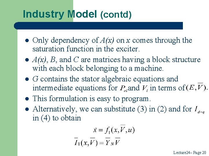
Industry Model (contd) l l l Only dependency of A(x) on x comes through the saturation function in the exciter. A(x), B, and C are matrices having a block structure with each block belonging to a machine. G contains the stator algebraic equations and intermediate equations for and in terms of This formulation is easy to program. Alternatively, we can substitute (3) in (2) and for in (4) to obtain Lecture 24– Page 20

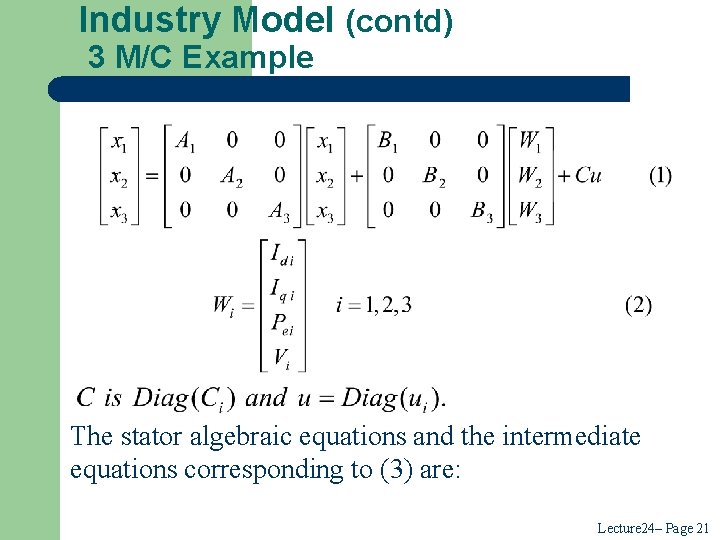
Industry Model (contd) 3 M/C Example The stator algebraic equations and the intermediate equations corresponding to (3) are: Lecture 24– Page 21

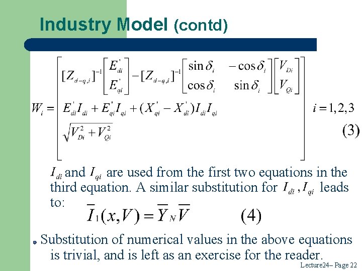
Industry Model (contd) and are used from the first two equations in the third equation. A similar substitution for leads to: Substitution of numerical values in the above equations is trivial, and is left as an exercise for the reader. Lecture 24– Page 22