ECE 576 POWER SYSTEM DYNAMICS AND STABILITY Lecture

ECE 576 POWER SYSTEM DYNAMICS AND STABILITY Lecture 29 Small Signal Analysis (SSA) of Power Systems Professor M. A. Pai Department of Electrical and Computer Engineering © 2000 University of Illinois Board of Trustees, All Rights Reserved

References Basic Text 1. P. W. Sauer & M. A. Pai ‘Power system dynamics and stability’. Prentice Hall 1998. 2. References 3. P. Kundur. ‘Power system stability and control’. Mc Graw Hill 1994. K. R. Padiyar. ‘Power system dynamics and control’ John Wiley and sons (Asia) 1996. M. Ilic and J. Zaborszky. ‘Dynamics and control of large electric power systems’ Wiley – Interscience 2000. Graham Rogers. ‘Power system oscillations’ Kluwer Academic Publishers 2000. “Analysis & control of P. S. oscillations”. CIGRE Committee 38 Task Force 07 of Advisory group 01, Dec 4. 5. 6. 7. Lecture 29 – Page 1

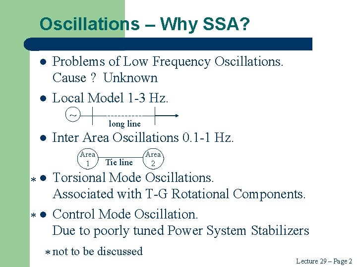
Oscillations – Why SSA? l l Problems of Low Frequency Oscillations. Cause ? Unknown Local Model 1 -3 Hz. ~ l long line Inter Area Oscillations 0. 1 -1 Hz. Area 1 Tie line Area 2 * l Torsional Mode Oscillations. *l Associated with T-G Rotational Components. Control Mode Oscillation. Due to poorly tuned Power System Stabilizers * not to be discussed Lecture 29 – Page 2

Techniques for SSA l Both DAE and DE models are used. l In DAE models, the network equations can be either - Power Balance Form OR -Current Balance Form l Industry favors a numerical approach (DAE). l In DAE Models, after linearizing, the algebraic equations are eliminated to compute eigen values. l Eigen values, eigen vectors of the linear system give lots of insight. Lecture 29 – Page 3

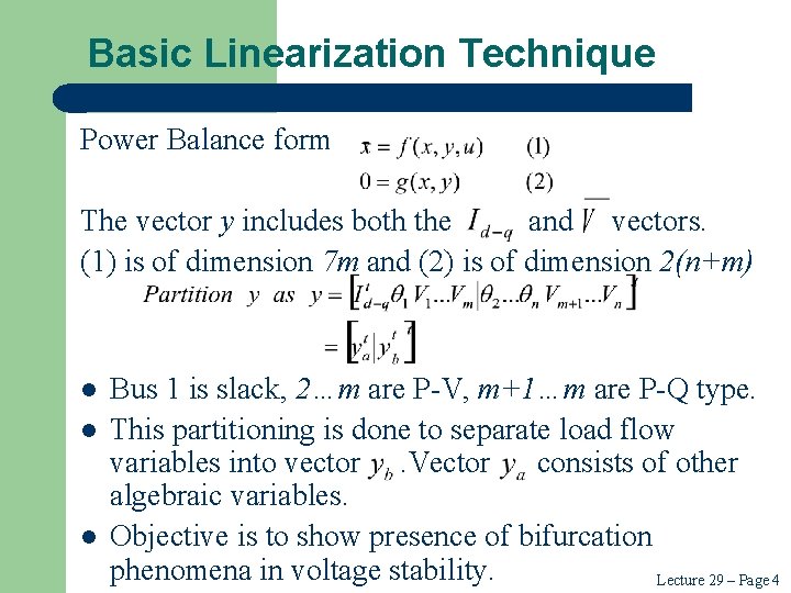
Basic Linearization Technique Power Balance form The vector y includes both the and vectors. (1) is of dimension 7 m and (2) is of dimension 2(n+m) l l l Bus 1 is slack, 2…m are P-V, m+1…m are P-Q type. This partitioning is done to separate load flow variables into vector. Vector consists of other algebraic variables. Objective is to show presence of bifurcation phenomena in voltage stability. Lecture 29 – Page 4

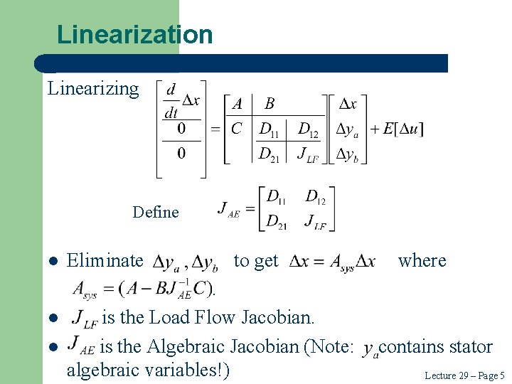
Linearization Linearizing Define l l l Eliminate to get . is the Load Flow Jacobian. is the Algebraic Jacobian (Note: algebraic variables!) where contains stator Lecture 29 – Page 5

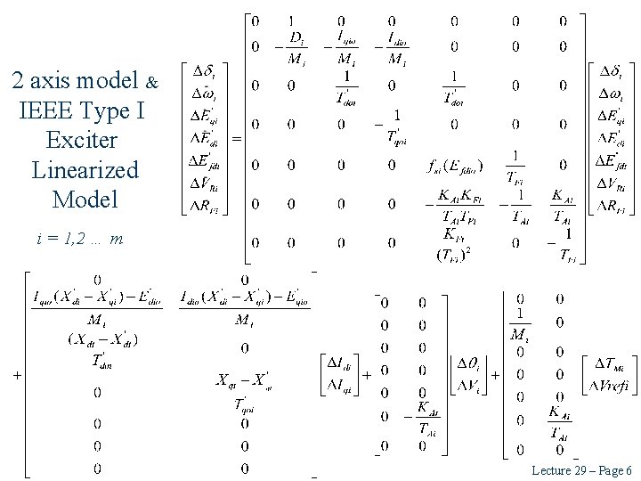
2 axis model & IEEE Type I Exciter Linearized Model i = 1, 2 … m Lecture 29 – Page 6

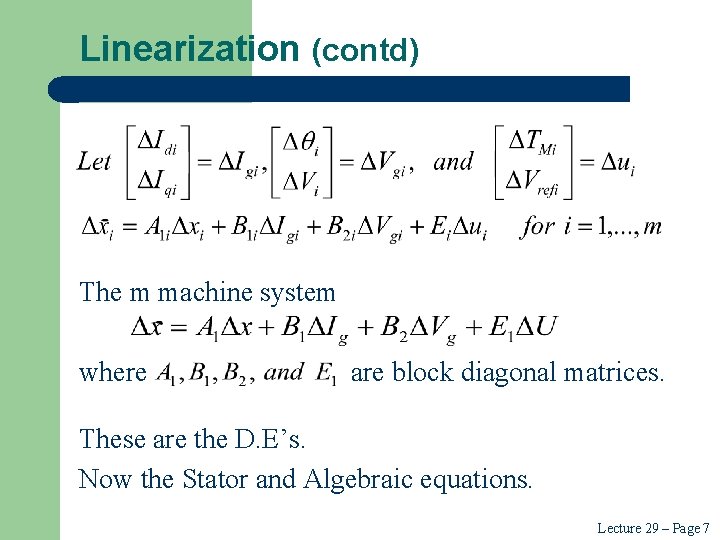
Linearization (contd) The m machine system where are block diagonal matrices. These are the D. E’s. Now the Stator and Algebraic equations. Lecture 29 – Page 7

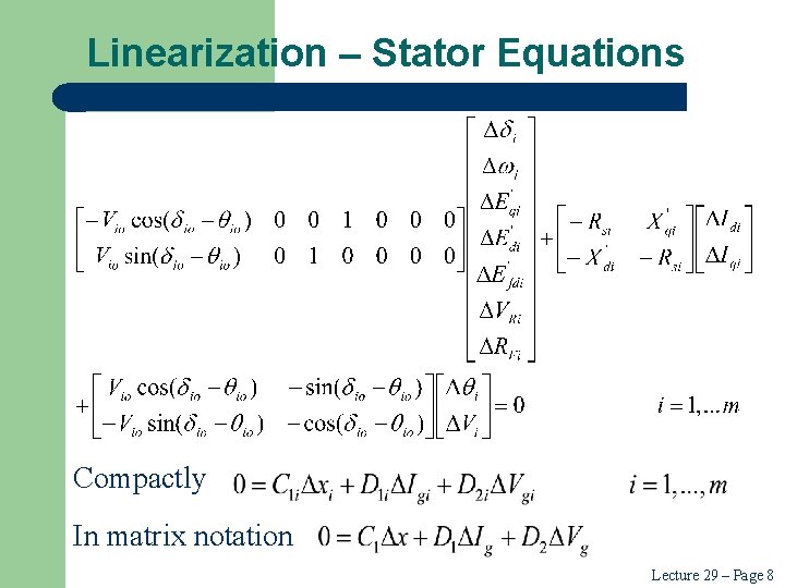
Linearization – Stator Equations Compactly In matrix notation Lecture 29 – Page 8

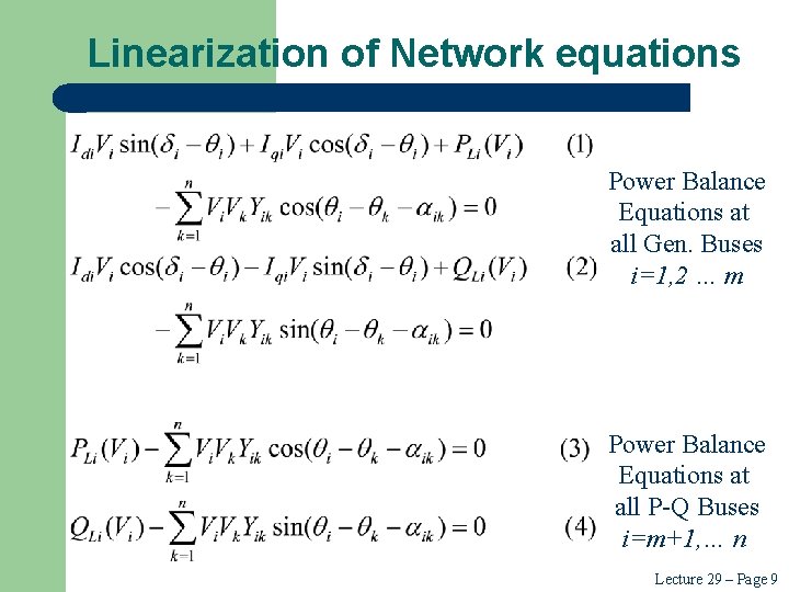
Linearization of Network equations Power Balance Equations at all Gen. Buses i=1, 2 … m Power Balance Equations at all P-Q Buses i=m+1, … n Lecture 29 – Page 9

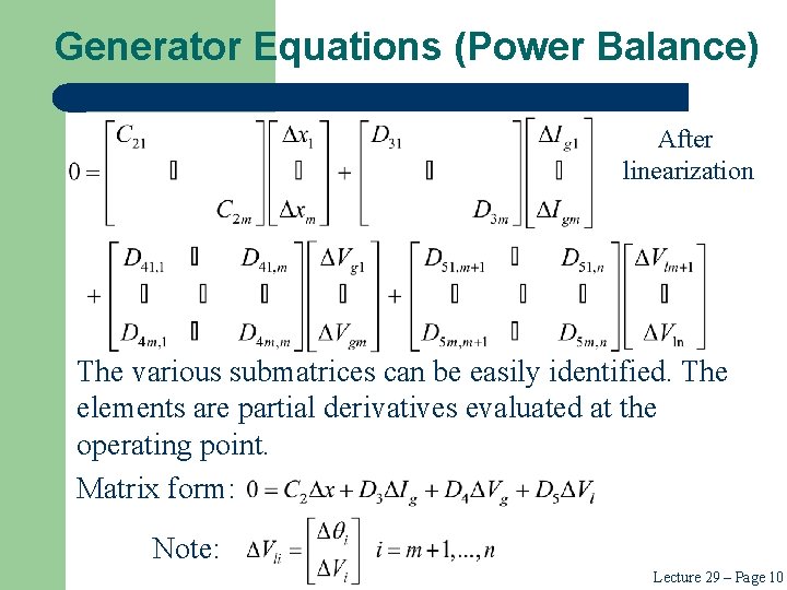
Generator Equations (Power Balance) After linearization The various submatrices can be easily identified. The elements are partial derivatives evaluated at the operating point. Matrix form: Note: Lecture 29 – Page 10

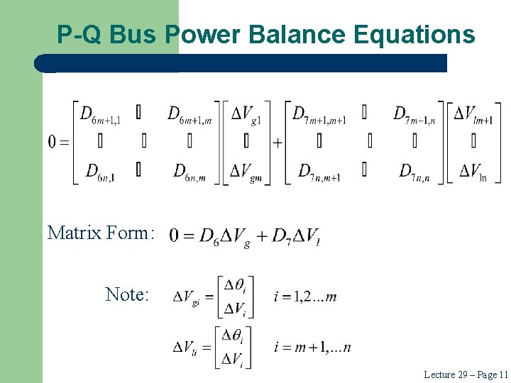
P-Q Bus Power Balance Equations Matrix Form: Note: Lecture 29 – Page 11

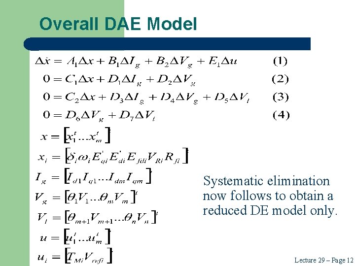
Overall DAE Model Systematic elimination now follows to obtain a reduced DE model only. Lecture 29 – Page 12

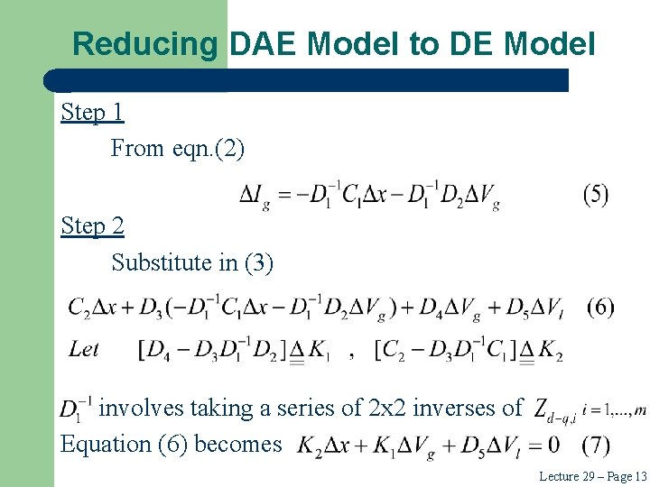
Reducing DAE Model to DE Model Step 1 From eqn. (2) Step 2 Substitute in (3) involves taking a series of 2 x 2 inverses of Equation (6) becomes Lecture 29 – Page 13

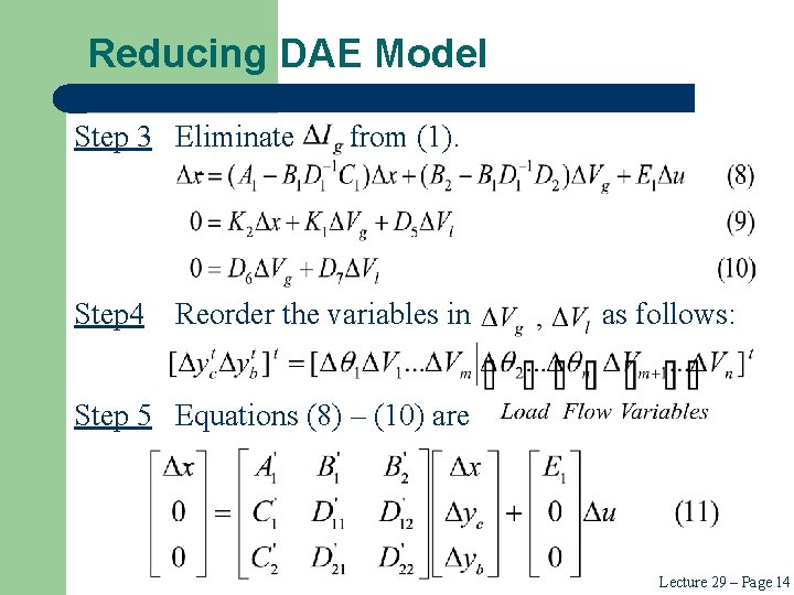
Reducing DAE Model Step 3 Eliminate Step 4 from (1). Reorder the variables in as follows: Step 5 Equations (8) – (10) are Lecture 29 – Page 14

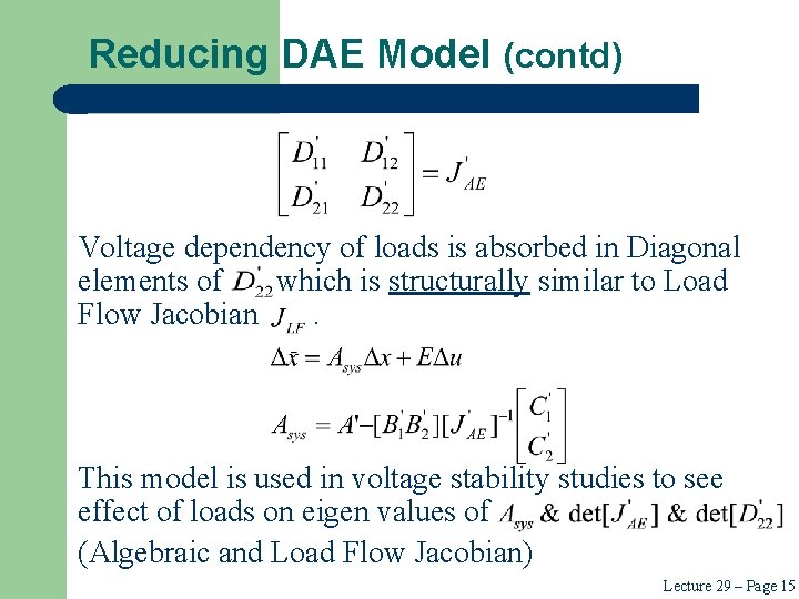
Reducing DAE Model (contd) Voltage dependency of loads is absorbed in Diagonal elements of which is structurally similar to Load Flow Jacobian. This model is used in voltage stability studies to see effect of loads on eigen values of (Algebraic and Load Flow Jacobian) Lecture 29 – Page 15

Reference angles l As in non-linear simulation, the order of D. E can be reduced to 7 m-1 instead of 7 m. l This mainly suppresses the zero eigen value in the original system. l To do it systematically proceed as follows. l Select one machine angle as reference angle. Lecture 29 – Page 16

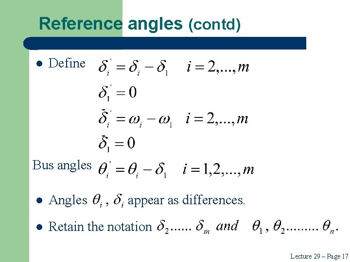
Reference angles (contd) l Define Bus angles l Angles appear as differences. l Retain the notation Lecture 29 – Page 17

Reference angles (contd) l Delete D. E corresponding to in (11). l Delete the column corresponding to l Replace l This means “mechanically” put a-1 in the inter sections of the rows corresponding to and corresponding to. in in (11). Lecture 29 – Page 18

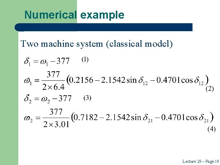
Numerical example Two machine system (classical model) Lecture 29 – Page 19

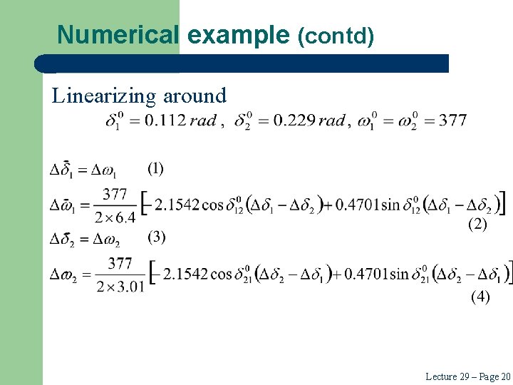
Numerical example (contd) Linearizing around Lecture 29 – Page 20

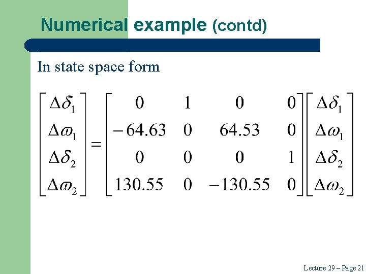
Numerical example (contd) In state space form Lecture 29 – Page 21

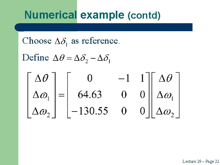
Numerical example (contd) Choose as reference. Define Lecture 29 – Page 22