ECE 576 Power System Dynamics and Stability Lecture

ECE 576 – Power System Dynamics and Stability Lecture 19: Multimachine Simulation Prof. Tom Overbye Dept. of Electrical and Computer Engineering University of Illinois at Urbana-Champaign overbye@illinois. edu 1

Announcements • • Read Chapter 7 Homework 6 is due on Tuesday April 15 A useful reference is B. Stott, "Power System Dynamic Response Calculations, " Proc. IEEE, vol. 67, pp. 219241 Another key reference is J. M. Undrill, "Structure in the Computation of Power-System Nonlinear Dynamic Response, " IEEE Trans. Power App. and Syst. , vol. 88, pp. 1 -6, January 1969. 2

Angle Reference • • The initial angles are given by the angles from the power flow, which are based on the slack bus's angle As presented the transient stability angles are with respect to a synchronous reference frame – Sometimes this is fine, such as for either shorter studies, or • ones in which there is little speed variation – Oftentimes this is not best since the when the frequencies are not nominal, the angles shift from the reference frame Other reference frames can be used, such as with respect to a particular generator's value, which mimics the power flow approach; the selected reference has no impact on the solution 3

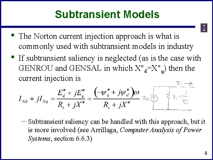
Subtransient Models • • The Norton current injection approach is what is commonly used with subtransient models in industry If subtransient saliency is neglected (as is the case with GENROU and GENSAL in which X"d=X"q) then the current injection is – Subtransient saliency can be handled with this approach, but it is more involved (see Arrillaga, Computer Analysis of Power Systems, section 6. 6. 3) 4

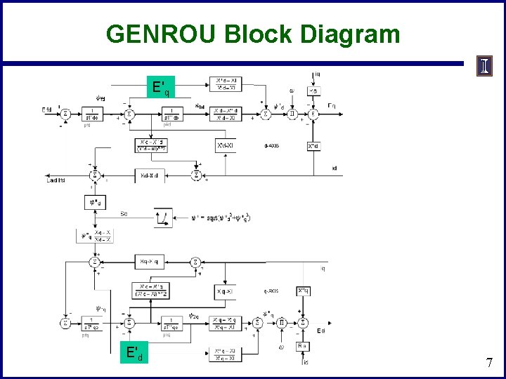
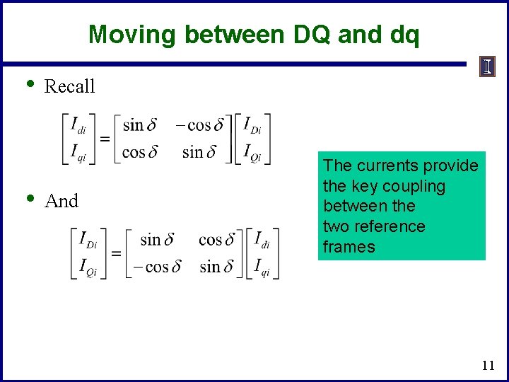
Subtransient Models • • Note, the values here are on the dq reference frame We can now extend the approach introduced for the classical machine model to subtransient models Initialization is as before, which gives the d's and other state values Each time step is as before, except we use the d's for each generator to transfer values between the network reference frame and each machine's dq reference frame – The currents provide the coupling 5

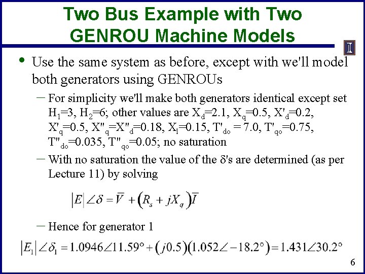
Two Bus Example with Two GENROU Machine Models • Use the same system as before, except with we'll model both generators using GENROUs – For simplicity we'll make both generators identical except set H 1=3, H 2=6; other values are Xd=2. 1, Xq=0. 5, X'd=0. 2, X'q=0. 5, X"q=X"d=0. 18, Xl=0. 15, T'do = 7. 0, T'qo=0. 75, T"do=0. 035, T"qo=0. 05; no saturation – With no saturation the value of the d's are determined (as per Lecture 11) by solving – Hence for generator 1 6

GENROU Block Diagram E'q E'd 7

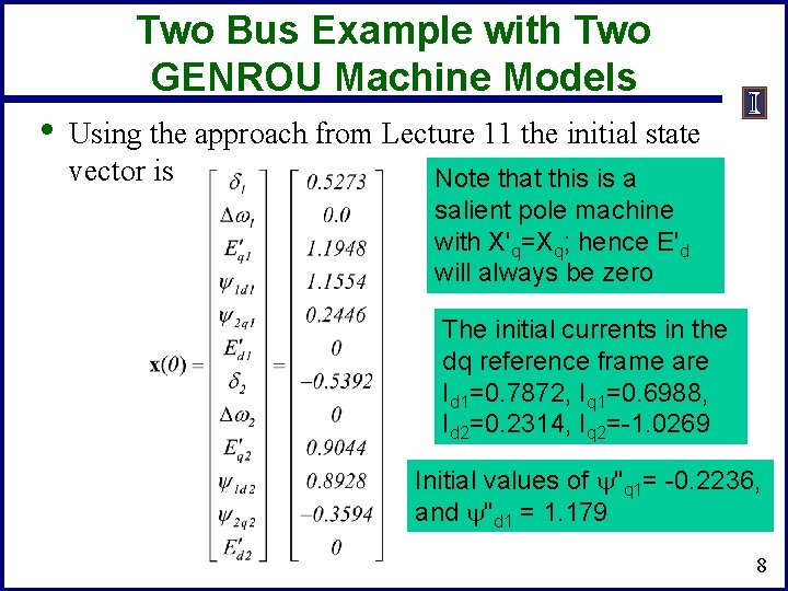
Two Bus Example with Two GENROU Machine Models • Using the approach from Lecture 11 the initial state vector is Note that this is a salient pole machine with X'q=Xq; hence E'd will always be zero The initial currents in the dq reference frame are Id 1=0. 7872, Iq 1=0. 6988, Id 2=0. 2314, Iq 2=-1. 0269 Initial values of "q 1= -0. 2236, and "d 1 = 1. 179 8

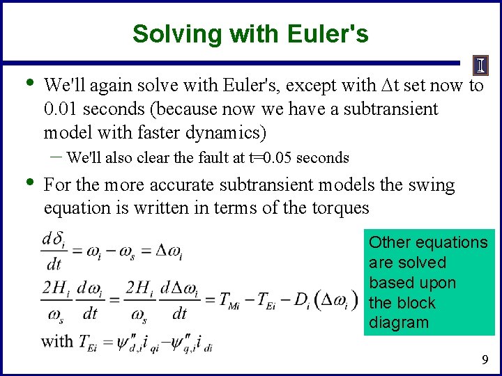
Solving with Euler's • • We'll again solve with Euler's, except with Dt set now to 0. 01 seconds (because now we have a subtransient model with faster dynamics) – We'll also clear the fault at t=0. 05 seconds For the more accurate subtransient models the swing equation is written in terms of the torques Other equations are solved based upon the block diagram 9

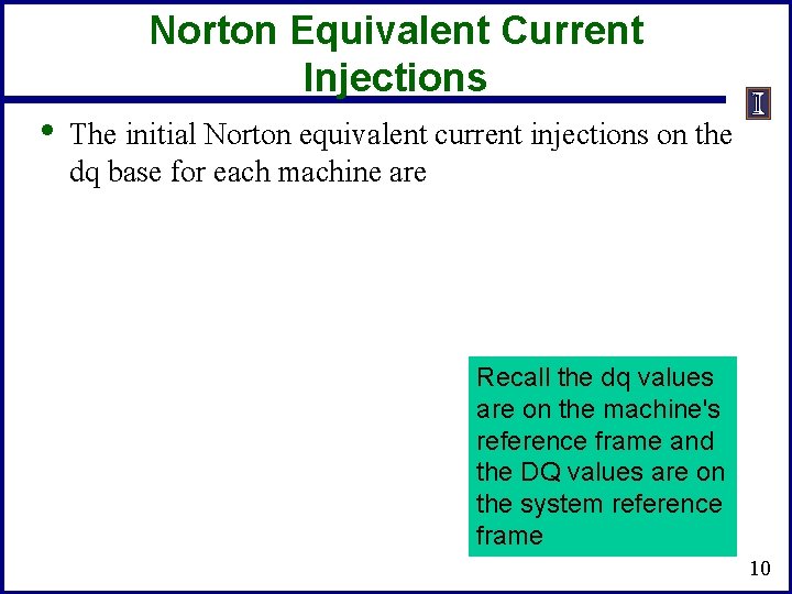
Norton Equivalent Current Injections • The initial Norton equivalent current injections on the dq base for each machine are Recall the dq values are on the machine's reference frame and the DQ values are on the system reference frame 10

Moving between DQ and dq • • Recall And The currents provide the key coupling between the two reference frames 11

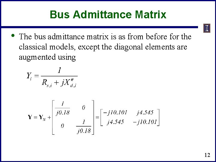
Bus Admittance Matrix • The bus admittance matrix is as from before for the classical models, except the diagonal elements are augmented using 12

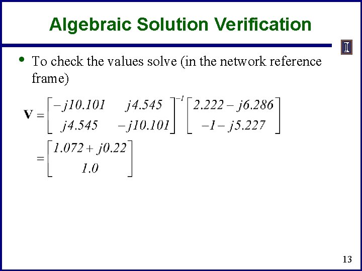
Algebraic Solution Verification • To check the values solve (in the network reference frame) 13

Results • The below graph shows the results for four seconds of simulation, using Euler's with Dt=0. 01 seconds Power. World case is B 2_GENROU_2 GEN_EULER 14

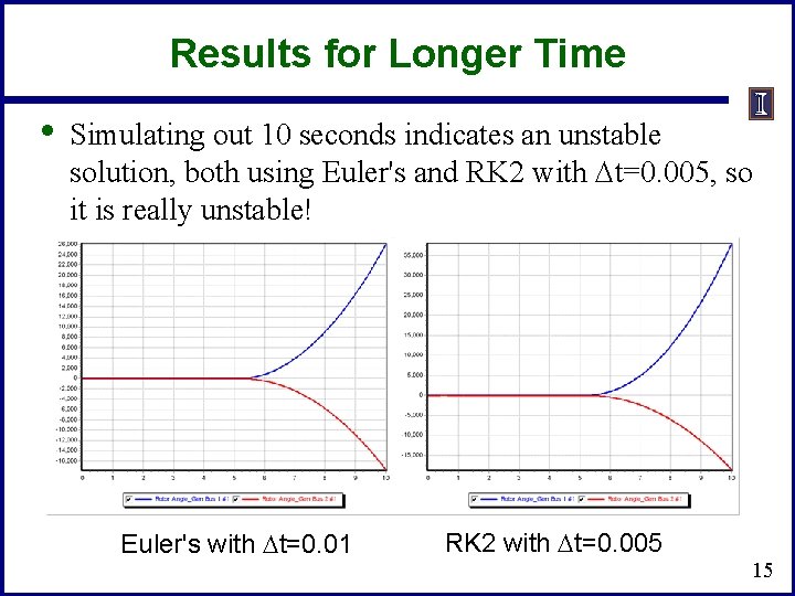
Results for Longer Time • Simulating out 10 seconds indicates an unstable solution, both using Euler's and RK 2 with Dt=0. 005, so it is really unstable! Euler's with Dt=0. 01 RK 2 with Dt=0. 005 15

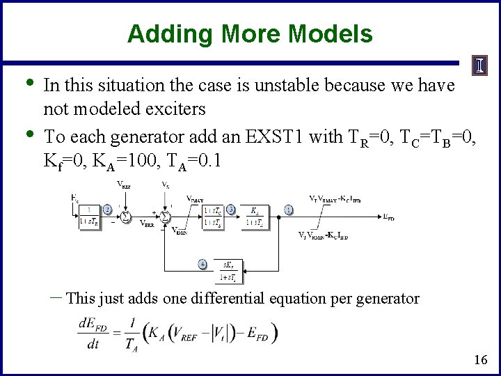
Adding More Models • • In this situation the case is unstable because we have not modeled exciters To each generator add an EXST 1 with TR=0, TC=TB=0, Kf=0, KA=100, TA=0. 1 – This just adds one differential equation per generator 16

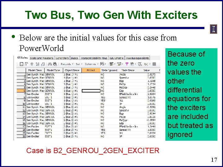
Two Bus, Two Gen With Exciters • Below are the initial values for this case from Power. World Because of the zero values the other differential equations for the exciters are included but treated as ignored Case is B 2_GENROU_2 GEN_EXCITER 17

Viewing the States • Power. World allows one to single-step through a solution, showing the f(x) and the K 1 values – This is mostly used for education or model debugging Derivatives shown are evaluated at the end of the time step 18

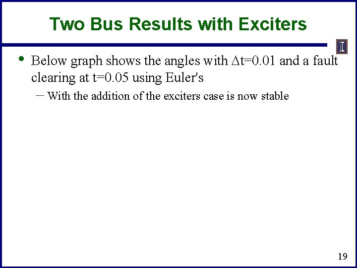
Two Bus Results with Exciters • Below graph shows the angles with Dt=0. 01 and a fault clearing at t=0. 05 using Euler's – With the addition of the exciters case is now stable 19

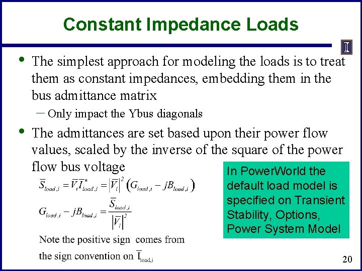
Constant Impedance Loads • • The simplest approach for modeling the loads is to treat them as constant impedances, embedding them in the bus admittance matrix – Only impact the Ybus diagonals The admittances are set based upon their power flow values, scaled by the inverse of the square of the power flow bus voltage In Power. World the default load model is specified on Transient Stability, Options, Power System Model 20

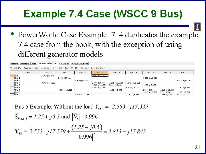
Example 7. 4 Case (WSCC 9 Bus) • Power. World Case Example_7_4 duplicates the example 7. 4 case from the book, with the exception of using different generator models 21

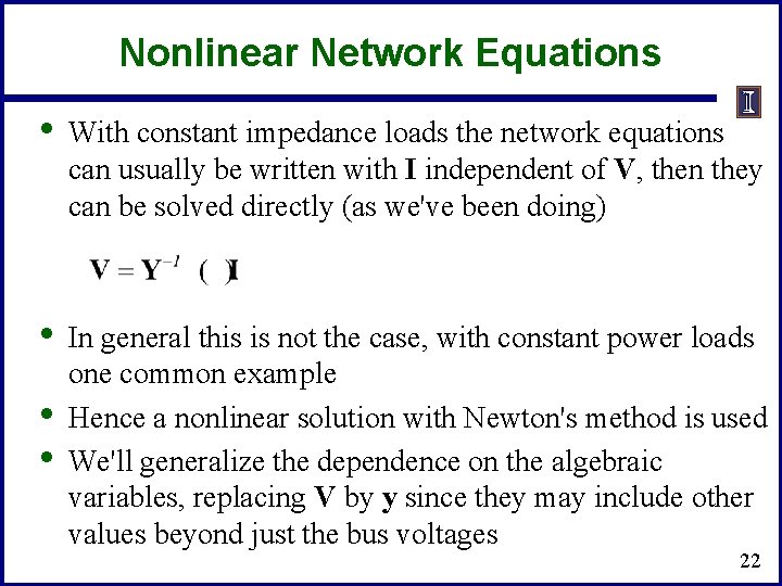
Nonlinear Network Equations • With constant impedance loads the network equations can usually be written with I independent of V, then they can be solved directly (as we've been doing) • In general this is not the case, with constant power loads one common example Hence a nonlinear solution with Newton's method is used We'll generalize the dependence on the algebraic variables, replacing V by y since they may include other values beyond just the bus voltages • • 22

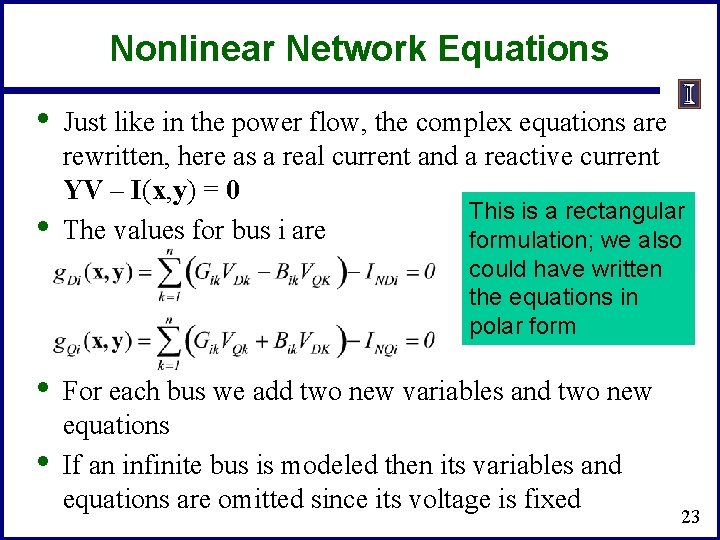
Nonlinear Network Equations • • Just like in the power flow, the complex equations are rewritten, here as a real current and a reactive current YV – I(x, y) = 0 This is a rectangular The values for bus i are formulation; we also could have written the equations in polar form • • For each bus we add two new variables and two new equations If an infinite bus is modeled then its variables and equations are omitted since its voltage is fixed 23

Nonlinear Network Equations • The network variables and equations are then 24

Nonlinear Network Equation Newton Solution 25

Network Equation Jacobian Matrix • The most computationally intensive part of the algorithm is determining and factoring the Jacobian matrix, J(y) 26

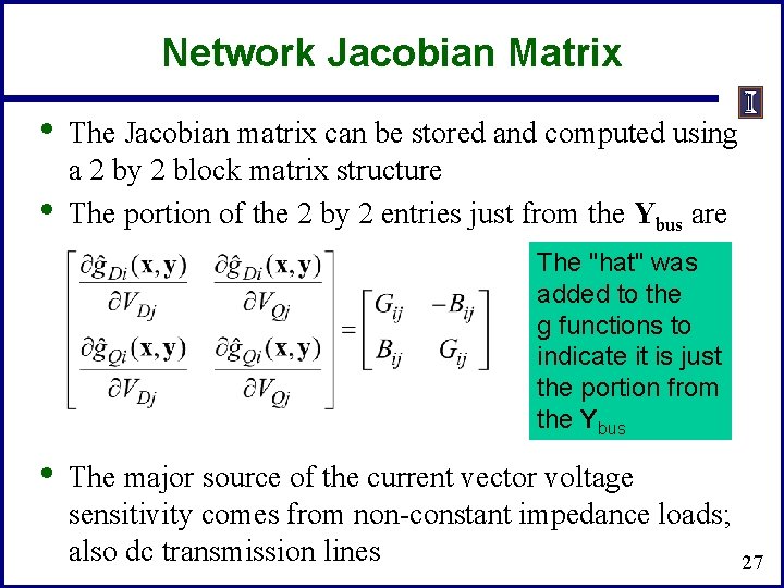
Network Jacobian Matrix • • The Jacobian matrix can be stored and computed using a 2 by 2 block matrix structure The portion of the 2 by 2 entries just from the Ybus are The "hat" was added to the g functions to indicate it is just the portion from the Ybus • The major source of the current vector voltage sensitivity comes from non-constant impedance loads; also dc transmission lines 27

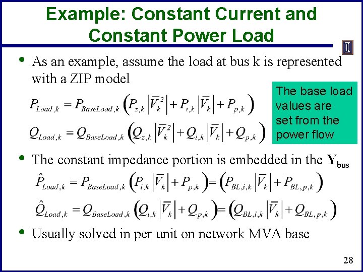
Example: Constant Current and Constant Power Load • As an example, assume the load at bus k is represented with a ZIP model The base load values are set from the power flow • The constant impedance portion is embedded in the Ybus • Usually solved in per unit on network MVA base 28

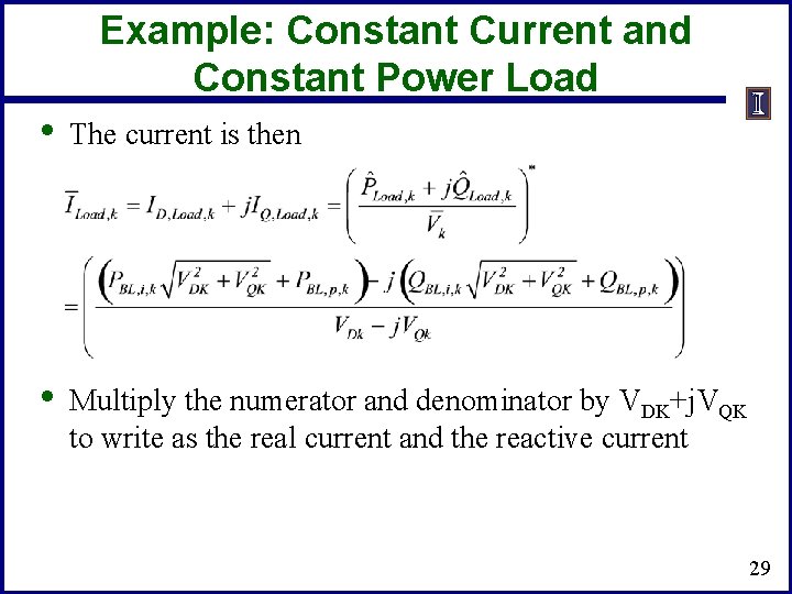
Example: Constant Current and Constant Power Load • The current is then • Multiply the numerator and denominator by VDK+j. VQK to write as the real current and the reactive current 29

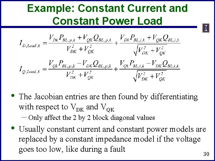
Example: Constant Current and Constant Power Load • • The Jacobian entries are then found by differentiating with respect to VDK and VQK – Only affect the 2 by 2 block diagonal values Usually constant current and constant power models are replaced by a constant impedance model if the voltage goes too low, like during a fault 30

Example: 7. 4. ZIP Case • Example 7. 4 is modified so the loads are represented by a model with 30% constant power, 30% constant current and 40% constant impedance – In Power. World load models can be entered in a number of different ways; a tedious but simple approach is to specify a model for each individual load • Right click on the load symbol to display the Load Options dialog, select Stability, and select WSCC to enter a ZIP model, in which p 1&q 1 are the normalized about of constant impedance load, p 2&q 2 the amount of constant current load, and p 3&q 3 the amount of constant power load Case is Example_7_4_ZIP 31

Example 7. 4. ZIP One-line 32

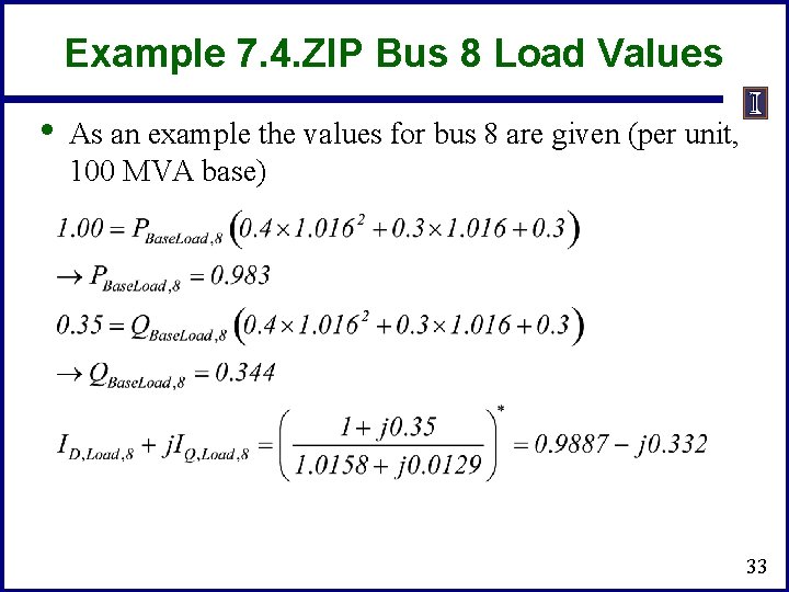
Example 7. 4. ZIP Bus 8 Load Values • As an example the values for bus 8 are given (per unit, 100 MVA base) 33

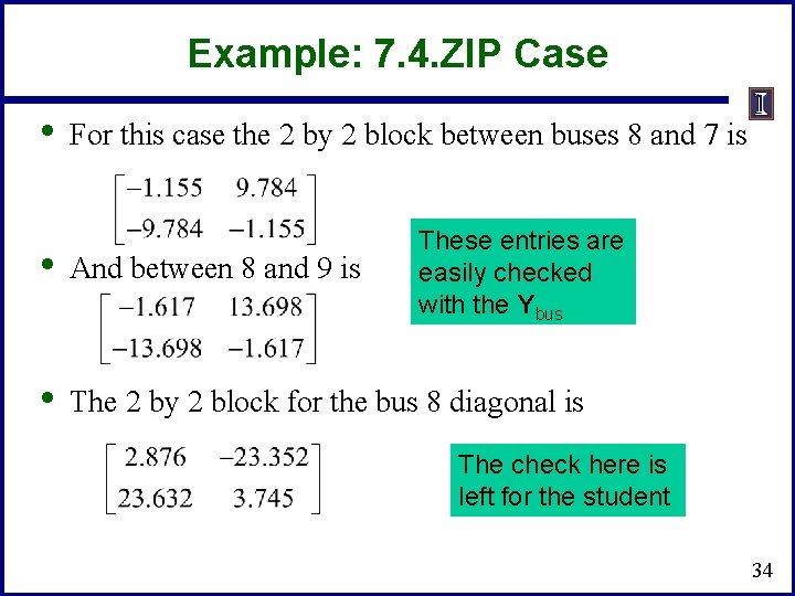
Example: 7. 4. ZIP Case • For this case the 2 by 2 block between buses 8 and 7 is These entries are easily checked with the Ybus • And between 8 and 9 is • The 2 by 2 block for the bus 8 diagonal is The check here is left for the student 34

Additional Comments • • • When coding Jacobian values, a good way to check that the entries are correct is to make sure that for a small perturbation about the solution the Newton's method has quadratic convergence When running the simulation the Jacobian is actually seldom rebuilt and refactored – If the Jacobian is not too bad it will still converge To converge Newton's method needs a good initial guess, which is usually the last time step solution – Convergence can be an issue following large system disturbances, such as a fault 35