ECE 565 VLSI Design Automation High Level Synthesis

ECE 565 – VLSI Design Automation High Level Synthesis Adapted from: EE 5301 - VLSI Design Automation I – © Kia Bazargan (slides used mainly from those of Kia Bazargan, Univ. of Minnesota, w/ a few modifications and additions by Shantanu Dutt; see p. 2 for full acknowledgements) EE 5301 - VLSI Design Automation 200

References and Copyright • Textbooks referred (none required) § [Mic 94] G. De Micheli “Synthesis and Optimization of Digital Circuits” Mc. Graw-Hill, 1994. • Slides used: (Modified originally by Kia Bazargan, U. Minn. , & subsequently by Shantanu Dutt, UIC, [ALAP schedule, list scheduling algorithms], when necessary) § [©Gupta] © Rajesh Gupta UC-Irvine http: //www. ics. uci. edu/~rgupta/ics 280. html § Ryan Kastner, UCSB § Sune Fallgaard Nielsen, Technical University of Denmark EE 5301 - VLSI Design Automation 201

High Level Synthesis (HLS) • The process of converting a high-level description of a design to a netlist § Input: o o High-level languages (e. g. , C) Behavioral hardware description languages (e. g. , VHDL) Structural HDLs (e. g. , VHDL) State diagrams / logic networks § Tools: o Parser o Library of modules § Constraints: o Area constraints (e. g. , # modules of a certain type) o Delay constraints (e. g. , set of operations should finish in l clock cycles) § Output: o Operation scheduling (time) and binding (resource) o Control generation and detailed interconnections EE 5301 - VLSI Design Automation 202

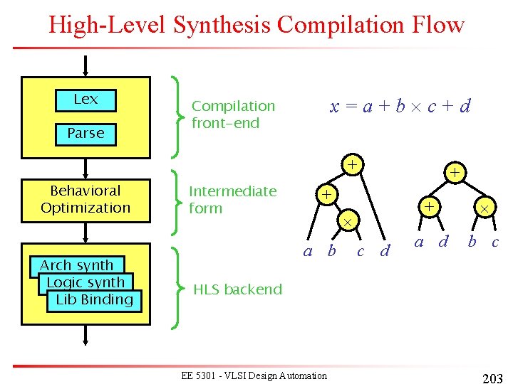
High-Level Synthesis Compilation Flow Lex Parse x=a+b c+d Compilation front-end + Behavioral Optimization Arch synth Logic synth Lib Binding Intermediate form + a b c d + + a d b c HLS backend EE 5301 - VLSI Design Automation 203

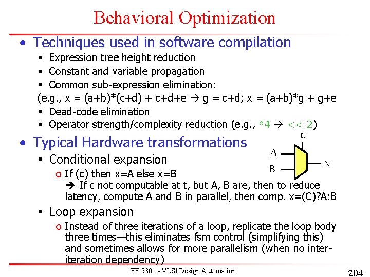
Behavioral Optimization • Techniques used in software compilation § Expression tree height reduction § Constant and variable propagation § Common sub-expression elimination: (e. g. , x = (a+b)*(c+d) + c+d+e g = c+d; x = (a+b)*g + g+e § Dead-code elimination § Operator strength/complexity reduction (e. g. , *4 << 2) c • Typical Hardware transformations § Conditional expansion A B x o If (c) then x=A else x=B If c not computable at t, but A, B are, then to reduce latency, compute A and B in parallel, then comp. x=(C)? A: B § Loop expansion o Instead of three iterations of a loop, replicate the loop body three times—this eliminates fsm control (simplifying this) and sometimes allows for more parallelism (when no interiteration dependency) EE 5301 - VLSI Design Automation 204

Architectural Synthesis • Deals with “computational” behavioral descriptions § Behavior as sequencing graph (aka dependency graph, or data flow graph DFG) § Hardware resources as library elements § Constraints on operation timing § Constraints on hardware resource availability § Other Costs: Storage as registers, data transfer using wires • Objective § Generate a synchronous, single-phase clock circuit § Might have multiple feasible solutions (explore tradeoff) § Satisfy constraints, minimize objective: o Maximize performance subject to area constraint o Minimize area subject to performance constraints [©Gupta] EE 5301 - VLSI Design Automation 205

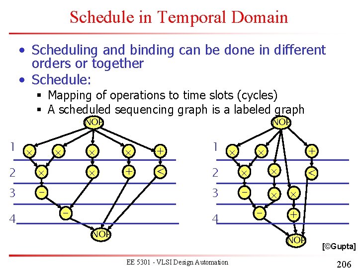
Schedule in Temporal Domain • Scheduling and binding can be done in different orders or together • Schedule: § Mapping of operations to time slots (cycles) § A scheduled sequencing graph is a labeled graph NOP 1 2 3 - 4 NOP + 1 + < 2 3 - NOP 4 + - < + NOP EE 5301 - VLSI Design Automation [©Gupta] 206

Operation Types & Binding • For each operation, define its type. • For each resource, define a resource type, and a delay (in terms of # cycles) • b is a function that maps an operation to a resource type that can implement it § b : V {1, 2, . . . , nres}. • More general case: § A resource type may implement more than one operation type (e. g. , ALU) • Resource binding: § Map each operation to a resource with the same type § Might have multiple options (different speed/power types)—module selection [©Gupta] EE 5301 - VLSI Design Automation 207

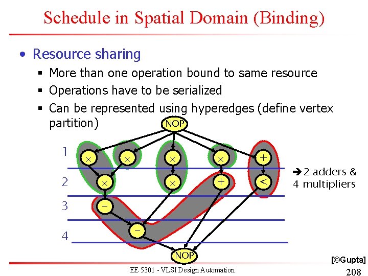
Schedule in Spatial Domain (Binding) • Resource sharing § More than one operation bound to same resource § Operations have to be serialized § Can be represented using hyperedges (define vertex NOP partition) 1 2 3 - 4 + + < 2 adders & 4 multipliers NOP EE 5301 - VLSI Design Automation [©Gupta] 208

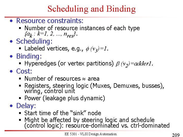
Scheduling and Binding • Resource constraints: § Number of resource instances of each type {ak : k=1, 2, . . . , nres}. • Scheduling: § Labeled vertices, e. g. , f (v 3)=1. • Binding: § Hyperedges (or vertex partitions) b (v 2)=adder 1. • Cost: § Number of resources area Resource dominated § Registers, steering logic (Muxes, Demuxes, busses), wiring, control unit § Power (leakage plus dynamic) Control dominated • Delay: § Start time of the “sink” node § Might be affected by steering logic and schedule (control logic): resource-dominated vs. ctrl-dominated EE 5301 - VLSI Design Automation 209

Architectural Optimization • Optimization in view of design space flexibility • A multi-criteria optimization problem: § Determine schedule f and binding b. § Under area A, power P, latency l and cycle time t objectives • Traditional Goals: § Min area: solve for minimal binding/resources § Min latency: solve for minimum l scheduling • Order of scheduling and binding? § Apply either one (scheduling, binding) first § Do both together! [©Gupta] EE 5301 - VLSI Design Automation 210

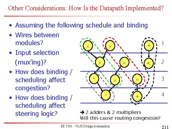
Other Considerations: How Is the Datapath Implemented? • Assuming the following schedule and binding • Wires between modules? + • Input selection (mux’ing)? < • How does binding / scheduling affect congestion? + • How does binding / scheduling affect 2 adders & 2 multipliers steering logic? 1 2 3 4 Will this cause routing congestion? EE 5301 - VLSI Design Automation 211

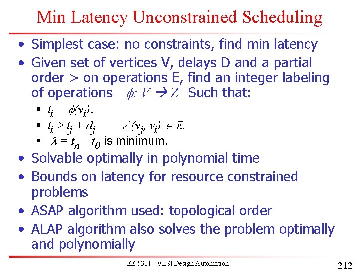
Min Latency Unconstrained Scheduling • Simplest case: no constraints, find min latency • Given set of vertices V, delays D and a partial order > on operations E, find an integer labeling of operations f: V Z+ Such that: § § § ti = f(vi). ti tj + dj (vj, vi) E. l = tn – t 0 is minimum. • Solvable optimally in polynomial time • Bounds on latency for resource constrained problems • ASAP algorithm used: topological order • ALAP algorithm also solves the problem optimally and polynomially EE 5301 - VLSI Design Automation 212

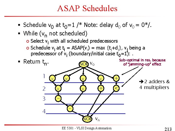
ASAP Schedules § Schedule v 0 at t 0=1 /* Note: delay d 0 of v 0 = 0*/. § While (vn not scheduled) o Select vi with all scheduled predecessors o Schedule vi at ti = ASAP(vi) = max {tj+dj}, vj being a predecessor of vi (boundary/initial case t 0=1): . § Return tn. 1 2 3 - 4 Sub-optimal in res. because of “jamming-up” effect NOP v 0 + + < 2 adders & 4 multipliers NOP vn EE 5301 - VLSI Design Automation 213

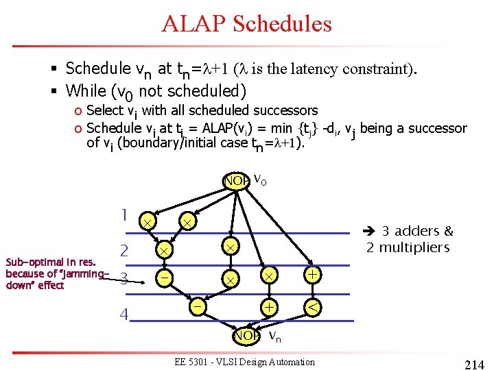
ALAP Schedules § Schedule vn at tn=l+1 (l is the latency constraint). § While (v 0 not scheduled) o Select vi with all scheduled successors o Schedule vi at ti = ALAP(vi) = min {tj} -di, vj being a successor of vi (boundary/initial case tn=l+1). NOP v 0 1 Sub-optimal in res. because of “jammingdown” effect 2 3 - 4 - 3 adders & 2 multipliers + + < NOP vn EE 5301 - VLSI Design Automation 214

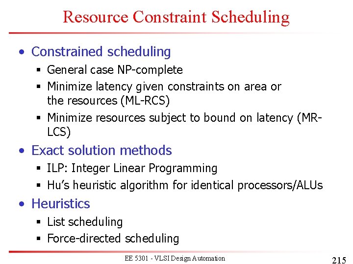
Resource Constraint Scheduling • Constrained scheduling § General case NP-complete § Minimize latency given constraints on area or the resources (ML-RCS) § Minimize resources subject to bound on latency (MRLCS) • Exact solution methods § ILP: Integer Linear Programming § Hu’s heuristic algorithm for identical processors/ALUs • Heuristics § List scheduling § Force-directed scheduling EE 5301 - VLSI Design Automation 215

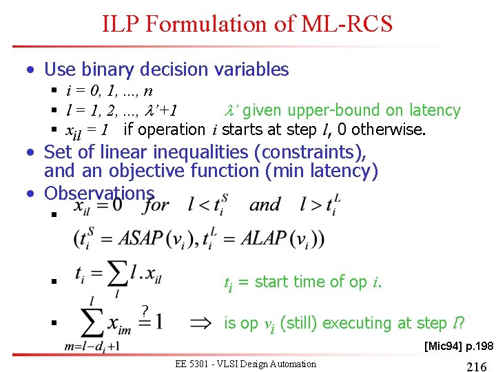
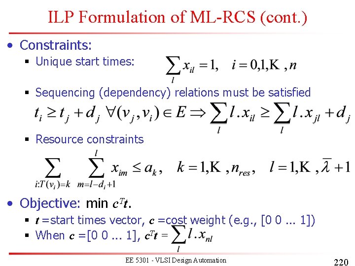
ILP Formulation of ML-RCS • Use binary decision variables § § § i = 0, 1, . . . , n l = 1, 2, . . . , l’+1 l’ given upper-bound on latency xil = 1 if operation i starts at step l, 0 otherwise. • Set of linear inequalities (constraints), and an objective function (min latency) • Observations § ti = start time of op i. § § ? is op vi (still) executing at step l? [Mic 94] p. 198 EE 5301 - VLSI Design Automation 216

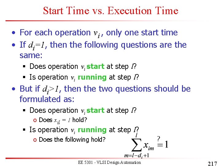
Start Time vs. Execution Time • For each operation vi , only one start time • If di=1, then the following questions are the same: § Does operation vi start at step l? § Is operation vi running at step l? • But if di>1, then the two questions should be formulated as: § Does operation vi start at step l? o Does xil = 1 hold? § Is operation vi running at step l? o Does the following hold? EE 5301 - VLSI Design Automation ? 217

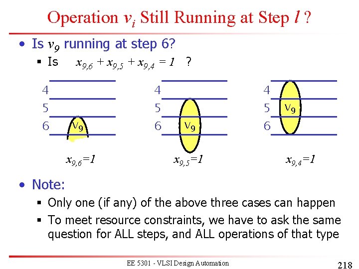
Operation vi Still Running at Step l ? • Is v 9 running at step 6? § Is 4 5 6 x 9, 6 + x 9, 5 + x 9, 4 = 1 ? v 9 x 9, 6=1 4 5 6 v 9 x 9, 5=1 4 5 6 v 9 x 9, 4=1 • Note: § Only one (if any) of the above three cases can happen § To meet resource constraints, we have to ask the same question for ALL steps, and ALL operations of that type EE 5301 - VLSI Design Automation 218

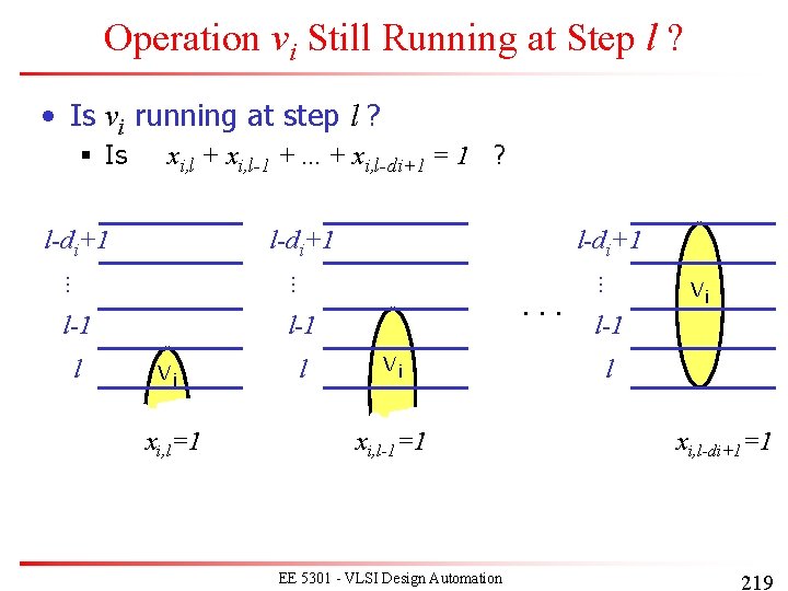
Operation vi Still Running at Step l ? • Is vi running at step l ? § Is xi, l + xi, l-1 +. . . + xi, l-di+1 = 1 ? l-di+1. . . l-1 l vi xi, l=1 l . . . vi xi, l-1=1 EE 5301 - VLSI Design Automation . . . l-1 l-di+1 vi l-1 l xi, l-di+1=1 219

ILP Formulation of ML-RCS (cont. ) • Constraints: § Unique start times: § Sequencing (dependency) relations must be satisfied § Resource constraints • Objective: min c. Tt. § t =start times vector, c =cost weight (e. g. , [0 0. . . 1]) § When c =[0 0. . . 1], c. Tt = EE 5301 - VLSI Design Automation 220

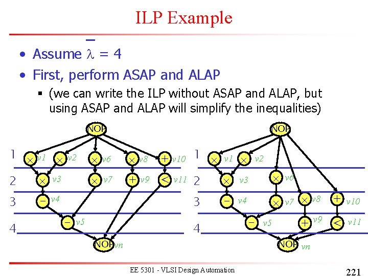
ILP Example • Assume l = 4 • First, perform ASAP and ALAP § (we can write the ILP without ASAP and ALAP, but using ASAP and ALAP will simplify the inequalities) NOP 1 v 1 2 v 3 3 - v 4 4 v 2 - NOP v 6 v 8 + v 10 1 v 7 + v 9 < 2 v 3 v 6 3 - v 4 v 7 v 5 NOP vn v 11 4 EE 5301 - VLSI Design Automation v 2 - v 5 v 8 + v 10 + v 9 < v 11 NOP vn 221

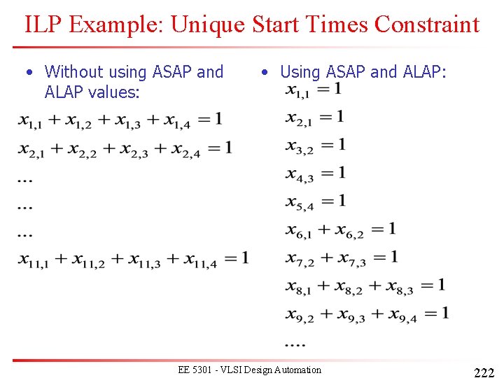
ILP Example: Unique Start Times Constraint • Without using ASAP and ALAP values: • Using ASAP and ALAP: EE 5301 - VLSI Design Automation 222

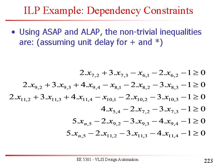
ILP Example: Dependency Constraints • Using ASAP and ALAP, the non-trivial inequalities are: (assuming unit delay for + and *) EE 5301 - VLSI Design Automation 223

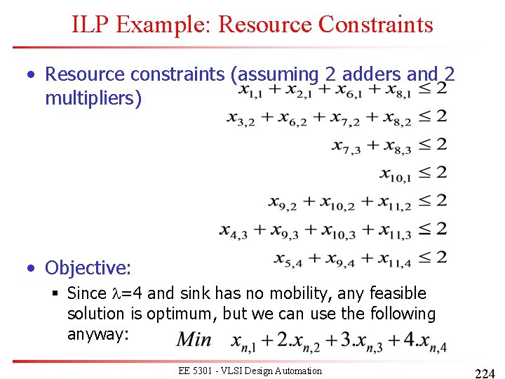
ILP Example: Resource Constraints • Resource constraints (assuming 2 adders and 2 multipliers) • Objective: § Since l=4 and sink has no mobility, any feasible solution is optimum, but we can use the following anyway: EE 5301 - VLSI Design Automation 224

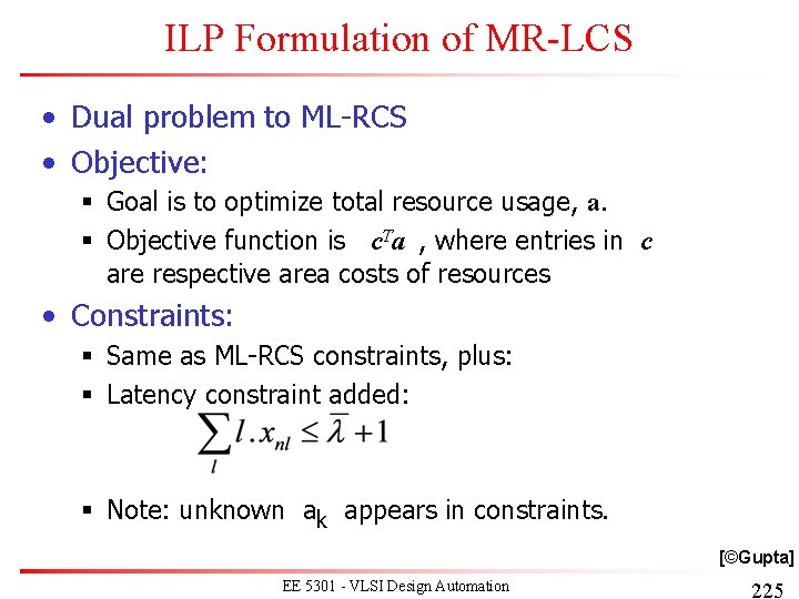
ILP Formulation of MR-LCS • Dual problem to ML-RCS • Objective: § Goal is to optimize total resource usage, a. § Objective function is c. Ta , where entries in c are respective area costs of resources • Constraints: § Same as ML-RCS constraints, plus: § Latency constraint added: § Note: unknown ak appears in constraints. [©Gupta] EE 5301 - VLSI Design Automation 225

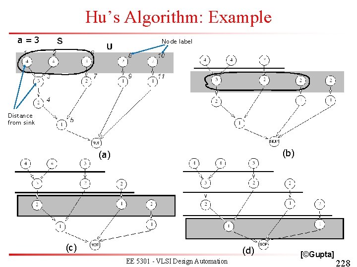
Hu’s Algorithm • Simple case of the scheduling problem § Operations of unit delay § Operations (and resources) of the same type • Hu’s algorithm § Greedy § Polynomial AND optimal § Computes lower bound on number of resources for a given latency OR: computes lower bound on latency subject to resource constraints • Basic idea: § Label operations based on their distances from the sink § Try to schedule nodes with higher labels first (i. e. , most “critical” operations have priority) [©Gupta] EE 5301 - VLSI Design Automation 226

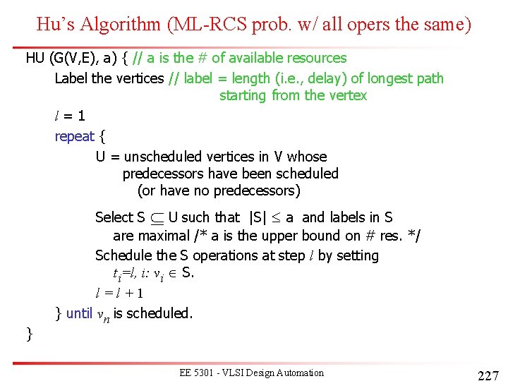
Hu’s Algorithm (ML-RCS prob. w/ all opers the same) HU (G(V, E), a) { // a is the # of available resources Label the vertices // label = length (i. e. , delay) of longest path starting from the vertex l=1 repeat { U = unscheduled vertices in V whose predecessors have been scheduled (or have no predecessors) } Select S U such that |S| a and labels in S are maximal /* a is the upper bound on # res. */ Schedule the S operations at step l by setting ti=l, i: vi S. l=l+1 } until vn is scheduled. EE 5301 - VLSI Design Automation 227

Hu’s Algorithm: Example a=3 Node label Distance from sink (b) (a) (c) (d) EE 5301 - VLSI Design Automation [©Gupta] 228

Hu’s Algorithm • Why is Hu’s optimal for all operations of the same type? • First note: In our earlier heuristic of breaking ties, the situation of two competing operations u 1, u 2 w/ the same label (distance to sink) having sibling output times to the most-critical children that affect the availability of their children w 1, w 2 differently will never occur, as all opers w/ higher labels than w 1, w 2 will be scheduled before either of w 1, w 2 (by the algorithm + all opers being the same type, this is also possible w/o wasting resource/FU execute cycles), making it possible to schedule w 1, w 2 at the same cc based on both the algorithm (note that w 1, w 2 also have the same label) and availability of resources (any of which w 1, w 2 can be scheduled on, as they are all of the same type— this may not be the case if w 1, w 2 are of different types , as then it is possible for an FU for one to be available when w 1, w 2 are, but not for the other). • We can prove by induction on the label of two nodes u 1, u 2 that if only one FU is available, scheduling either on it will result in the same solution in terms of the final latency (the induction step for label l = k is shown in the figure below). This argument can then be extended by a double induction on the number of nodes that have the same label and a triple induction on the number FUs available for them. EE 5301 - VLSI Design Automation [©Dutt] 229

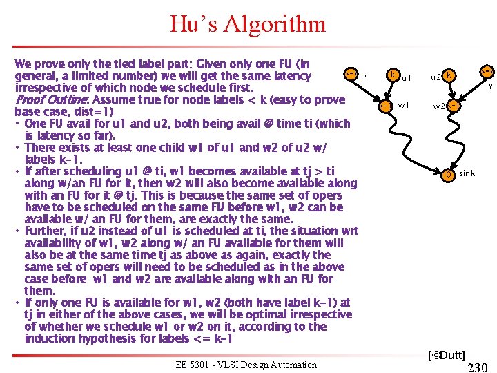
Hu’s Algorithm We prove only the tied label part: Given only one FU (in >=k general, a limited number) we will get the same latency irrespective of which node we schedule first. Proof Outline: Assume true for node labels < k (easy to prove base case, dist=1) • One FU avail for u 1 and u 2, both being avail @ time ti (which is latency so far). • There exists at least one child w 1 of u 1 and w 2 of u 2 w/ labels k-1. • If after scheduling u 1 @ ti, w 1 becomes available at tj > ti along w/an FU for it, then w 2 will also become available along with an FU for it @ tj. This is because the same set of opers have to be scheduled on the same FU before w 1, w 2 can be available w/ an FU for them, are exactly the same. • Further, if u 2 instead of u 1 is scheduled at ti, the situation wrt availability of w 1, w 2 along w/ an FU available for them will also be at the same time tj as above as again, exactly the same set of opers will need to be scheduled as in the above case before w 1 and w 2 are available along with an FU for them. • If only one FU is available for w 1, w 2 (both have label k-1) at tj in either of the above cases, we will be optimal irrespective of whether we schedule w 1 or w 2 on it, according to the induction hypothesis for labels <= k-1 EE 5301 - VLSI Design Automation x k u 1 k-1 w 1 >=k u 2 k y w 2 k-1 0 sink [©Dutt] 230

List Scheduling • Greedy algorithm for ML-RCS and MR-LCS § Extended Hu-type scheduling § Does NOT guarantee optimum solution • Similar to Hu’s algorithm § Operation selection decided by criticality § O(n log n ) time complexity • More general input § Resource constraints on different resource types EE 5301 - VLSI Design Automation 231

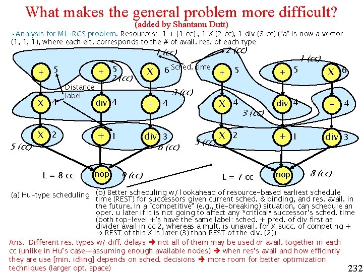
What makes the general problem more difficult? (added by Shantanu Dutt) • Analysis for ML-RCS problem. Resources: 1 + (1 cc) , 1 X (2 cc), 1 div (3 cc) (“a” is now a vector (1, 1, 1), where each elt. corresponds to the # of avail. res. of each type 2 (cc) 1 (cc) + 5 X 4 5 (cc) + Distance label X 2 L = 8 cc 5 2 (cc) div 4 + + 1 nop X 6 Sched. time 4 div 3 3 (cc) 6 (cc) 9 (cc) + 5 X 4 5 (cc) + 3 (cc) X 2 L = 7 cc 5 div 4 + 1 nop 1 (cc) X 6 + 4 div 3 8 (cc) (a) Hu-type scheduling (b) Better scheduling w/ lookahead of resource-based earliest schedule time (REST) for successors given current sched. & binding, and res. avail. in the future. In a “competitive” (e. g. , tie-breaking) situation, can schedule an oper. u later if it is not going to affect any *critical* successor’s sched. time (both top-level +’s have the same label: sched. + pred. of div first as divider avail in cc 2, whereas a mult. is unavail. for X succ. of competing + REST of this X is later (3) than REST of the div. (2)) Ans. Different res. types w/ diff. delays not all of them may be used or avail. together in each cc (unlike in Hu’s case—assuming enough available nodes) when res’s avail and how efficintly they are use [min. idling] depends on sched. decisions more room for better optimization techniques (larger opt. space) 232

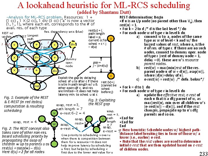
A lookahead heuristic for ML-RCS scheduling (added by Shantanu Dutt) • Analysis for ML-RCS problem. Resources: 1 + (1 cc) , 1 X (2 cc), 1 div (3 cc) (“a” is now a vector (1, 1, 1), where each elt. corresponds to the # of avail. res. of each type REST w/ update ro E-REST Longest path 1 label 1 2 + 5 Res. dependency arcs (blue) 1 2 (cc) 3 X 5 X 4 2 2 div 4 4 5 + 1 nop 6 X div rest(u) = i, path length label = p, u current cc for sched. = c < j – d(u) 3 4 + 4 5 dummy oper. node gap = j – (c+d(u)) div 3 Exploit the gap by delaying sched. of u to after c if there is a tie in path length w/ u & other opers @ c, and res. are limited—it does not help latency min. to sched. u at c v rest (v)= j (cannot be sched. before j) REST determination: Begin • If u is an i/p node (no parent other than V 0), then rest(u) = 1. • For k = 2 to d /* d is the last level */ do • For each node w of type r in level k do a) connect w to ar nodes of the same type as w of level < k and w/ the largest values of rest, where ar is the # of res. of type r. If there are no such nodes, connect to dummy oper. node of type r (rest of dummy node = 1, delay = 0). these are w’s resource parent nodes. b) rest(w) = max{min{rest of the res. parent node u of w + d(u)}, asap(w)}, where (d(u)=delay of u). c) e-rest(w) = rest(w) /* defn. below*/ • For k = d to 1 do • For each node w of type r in level k do a) update the effective rest, e-rest of Fig. 1: Example of the REST each u that is a dfg parent of w, as Fig. 3: Exploiting & E-REST (in red italics) max{rest(u), min over all children w’s the REST gap asap, rest =3, computation & resulting (e-rest(w)) – d(u))}, and if the rest path length = 7 changes, propagate up to u’s dfg scheduling asap, u e-rest: 6 -2 = 4 parents and so on. rest = 3, • End for v path asap, length • End for asap, rest = 4 rest=3 w asap, =7 End asap, e-rest = 6 Fig. 2: The REST concept also e-rest = 5 • New heuristic: Schedule nodes w/ highest pathtakes care of other non-res. distance label breaking ties in favor of those w/ a Give priority to scheduling v over u based scheduling priority by lower (i. e. , earlier) e-rest. when there is competition between propagating the asap of • Note that the rest values are used to determine them for a resource—it does not children w up to parents u as help improve latency by scheduling initial e-rest that are then updated based on e-rest(u) = asap(w) – d(u). u first, but helps by scheduling v of children nodes. Here d(u) = 2 for all nodes first due to the lower rest value for u 233

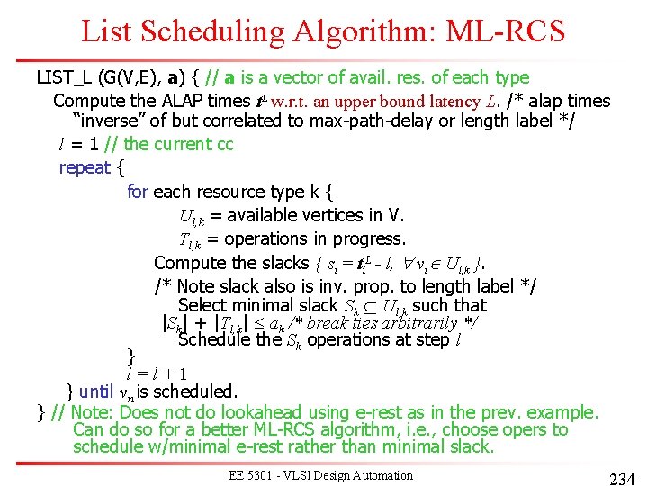
List Scheduling Algorithm: ML-RCS LIST_L (G(V, E), a) { // a is a vector of avail. res. of each type Compute the ALAP times t. L w. r. t. an upper bound latency L. /* alap times “inverse” of but correlated to max-path-delay or length label */ l = 1 // the current cc repeat { for each resource type k { Ul, k = available vertices in V. Tl, k = operations in progress. Compute the slacks { si = ti. L - l, vi Ul, k }. /* Note slack also is inv. prop. to length label */ Select minimal slack Sk Ul, k such that |Sk| + |Tl, k| ak /* break ties arbitrarily */ Schedule the Sk operations at step l } l=l+1 } until vn is scheduled. } // Note: Does not do lookahead using e-rest as in the prev. example. Can do so for a better ML-RCS algorithm, i. e. , choose opers to schedule w/minimal e-rest rather than minimal slack. EE 5301 - VLSI Design Automation 234

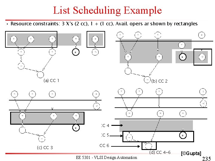
List Scheduling Example • Resource constraints: 3 X’s (2 cc), 1 + (1 cc). Avail. opers ar shown by rectangles * * (a) CC 1 (b) CC 2 * CC 4 CC 5 (c) CC 3 * CC 6 EE 5301 - VLSI Design Automation (d) CC 4 -6 [©Gupta] 235

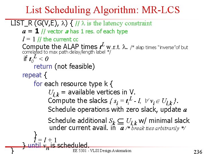
List Scheduling Algorithm: MR-LCS LIST_R (G(V, E), l) { // l is the latency constraint a = 1 // vector a has 1 res. of each type l = 1 // the current cc Compute the ALAP times t. L w. r. t. l. /* alap times “inverse”of but correlated to max path delay/length label */ if t 0 L < 0 return (not feasible) repeat { for each resource type k { Ul, k = available vertices in V. Compute the slacks { si = ti. L - l, vi Ul, k }. Schedule operations with zero slack, update a Schedule additional Sk Ul, k w/ minimal slack under current avail. in a /* break ties arbitrarily */ } } l=l+1 } until vn is scheduled. EE 5301 - VLSI Design Automation 236

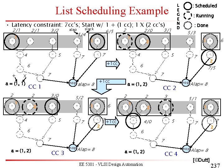
List Scheduling Example • Latency constraint: 7 cc’s; Start w/ 1 + (1 cc); 1 X (2 cc’s) 2/1 3/2 2/1 1 4 alap 5 slack 5/4 6/5 7 7 a = (1, 1) nop 3/0 2 1 alap= 8 5/3 a = (1, 2) 6 7 2 7/5 7 6 2 CC 2 3 2 1 nop Alap= 8 5/1 1 2 7 +1 cc 6 1 5 2 1 5 5 4/0 7 6 7 a = (1, 2) : Done 6 +1 cc 5/2 2 4 : Running 7 CC 1 2 : Scheduled 2 4 +1 cc 7 X 3/1 2/0 1 1 6 + 2 L E G E N D 2 7 7 CC 3 nop Alap= 8 a = (1, 2) EE 5301 - VLSI Design Automation CC 4 nop Alap= 8 [©Dutt] 237

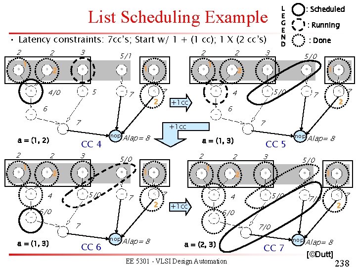
List Scheduling Example • Latency constraints: 7 cc’s; Start w/ 1 + (1 cc); 1 X (2 cc’s) 2 3 2 1 2 5/1 1 1 2 5 4/0 7 2 6 7 7 a = (1, 2) 2 CC 4 3 2 1 nop 5/0 4 6/0 2 1 2 7 7 +1 cc CC 5 3 nop 2 7 Alap= 8 5/0 1 2 5/0 4 7/0 6/0 7 a = (1, 3) 5/0 7 2 7 5/0 6 a = (1, 3) 1 2 : Done 1 4 +1 cc 5/0 : Running 2 +1 cc Alap= 8 3 2 : Scheduled L E G E N D 2 7 7/0 CC 6 nop Alap= 8 a = (2, 3) EE 5301 - VLSI Design Automation CC 7 nop Alap= 8 [©Dutt] 238

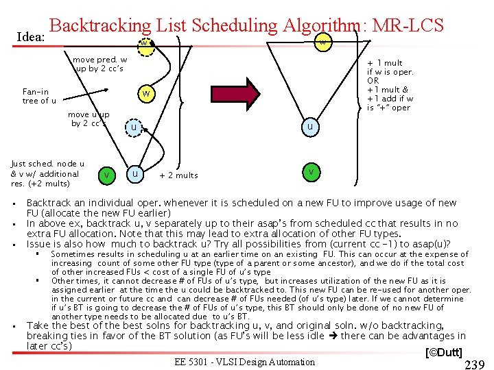
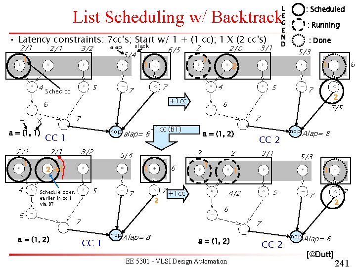
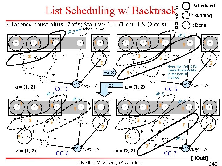
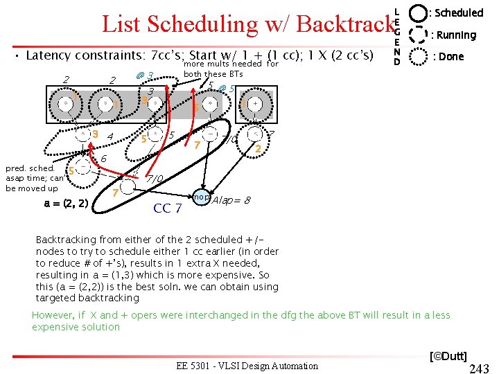
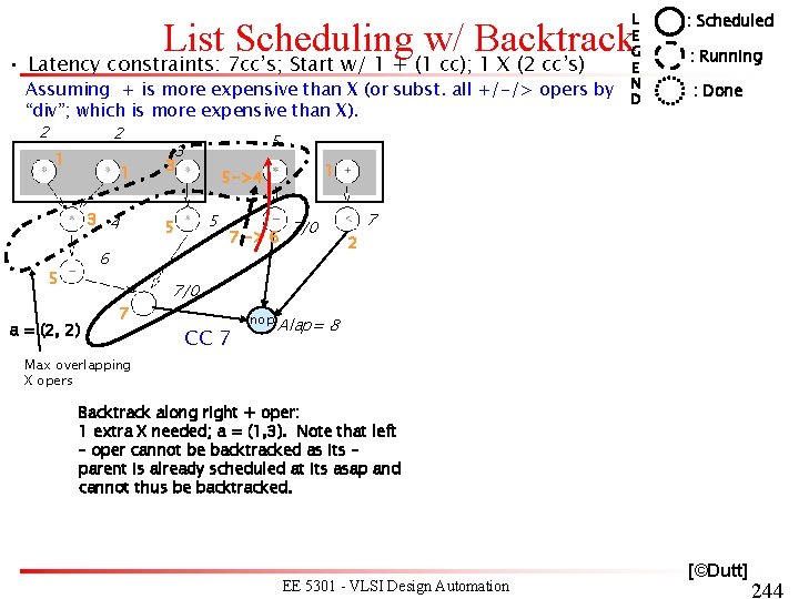
Idea: Backtracking List Scheduling Algorithm: MR-LCS w w move pred. w up by 2 cc’s Fan-in tree of u + 1 mult if w is oper. OR +1 mult & +1 add if w is “+” oper w move u up by 2 cc’s Just sched. node u & v w/ additional res. (+2 mults) v u u u + 2 mults v • Backtrack an individual oper. whenever it is scheduled on a new FU to improve usage of new FU (allocate the new FU earlier) • In above ex, backtrack u, v separately up to their asap’s from scheduled cc that results in no extra FU allocation. Note that this may lead to extra allocation of other FU types. • Issue is also how much to backtrack u? Try all possibilities from (current cc -1) to asap(u)? § § Sometimes results in scheduling u at an earlier time on an existing FU. This can occur at the expense of increasing count of some other FU type (type of a parent or some ancestor), and we do if the total cost of other increased FUs < cost of a single FU of u’s type Other times, it cannot decrease # of FUs of u’s type, but increases utilization of the new FU as it is assigned earlier at the time the u could be backtracked to. This new FU can be re-used for another oper. in the current or future cc and can decrease # of FUs needed (of u’s type) later. If we cannot determine if u’s BT is going to decrease the # of FUs of u’s type, this BT should only be done of no new FU of another type needs to be allocated due to u’s BT. • Take the best of the best solns for backtracking u, v, and original soln. w/o backtracking, breaking ties in favor of the BT solution (as FU’s will be less idle there can be advantages in later cc’s) EE 5301 - VLSI Design Automation [©Dutt] 239

Backtracking List Scheduling Algorithm: MR-LCS w w move pred. w LIST_R_BT (G(V, E), l’) { + 1 mult up by 2 cc’s a = 1, l=1 if w is Fan-in w Compute the ALAP times t. L. oper. tree of u OR if t 0 L < 0 move u up +1 mult u return (not feasible) by 2 cc’s u & +1 repeat { add if w for each resource type k { is “+” op u v v Ul, k = available vertices in V. + 2 mults L Compute the slacks { si = ti - l, vi Ul, k }. Just sched. node u & v w/ Schedule operations with 0 slack, upd. a additional res. (+2 mults) if a(k) is increased by an amount m > 0 { for each oper just scheduled { Backtrack along its fan-in tree to re-schedule itself its max-arrival time pred. as earlier as possible w/o increasing overall cost; Mark this oper. if CD = cost(res. k) - added cost of extra res. of other types needed for this >= 0; } Let S = the marked opers that have the highest m CDs for each oper in S in order of decreasing CDs { re-scheduled its fan-in tree as determined by above backtracking; /* may need to resolve conflicts w/ previous backtrackings */ update a } } /* if */ Schedule additional Sk Ul, k w/ minimal slack under a constraints } /* for */ l=l+1 } until vn is scheduled. } [©Dutt] EE 5301 - VLSI Design Automation 240

L E G E N D : Scheduled List Scheduling w/ Backtrack • Latency constraints: 7 cc’s; Start w/ 1 + (1 cc); 1 X (2 cc’s) 2/1 3/2 2/1 1 4 alap 5 Sched cc slack 5/4 6/5 7 7 a = (1, 1) CC 1 2/1 1 4 3/2 alap= 8 a = (1, 2) 5 2 6 1 5 a = (1, 2) 7 2 7/5 7 2 CC 2 3/1 2 1 nop Alap= 8 5/3 1 1 7 +1 cc 6 1 6 -1 cc (BT) 5/4 2 1 6 5/3 7 nop Schedule oper. earlier in cc 1 via BT : Done 2 4 +1 cc 7 X 3/1 2/0 1 1 6 + 2 : Running 5 4/2 7 6 7 2 7 7 CC 1 nop Alap= 8 a = (1, 2) EE 5301 - VLSI Design Automation CC 2 nop Alap= 8 [©Dutt] 241

: Scheduled L E G E N D List Scheduling w/ Backtrack • Latency constraints: 7 cc’s; Start w/ 1 + (1 cc); 1 X (2 cc’s) 2 2 1 1 @3 3/0 sched. time 3 7 2 2 1 1 3 4 5 @3 CC 3 Alap= 8 3 5 7 2 2 CC 6 nop Alap= 8 1 3 4 7 @3 5/0 EE 5301 - VLSI Design Automation 7 7 2 Note: No 3’rd X FU needed here unlike in the non-BT method. CC 5 3 nop @5 3 5 5 7/0 7 Alap= 8 5 1 5 7 6 a = (2, 2) 1 5 5 a = (1, 2) 5 7 3 7 1 1 5 5 : Done @ 5 5/0 3 6/1 2 6 a = (1, 2) +1 cc @ 55 3/0 5 nop 1 3 4 +2 cc 7 a = (1, 2) 7 2 6 2 1 1 5 3 4/1 2 5/2 : Running 7/0 2 7 @7 CC 7 nop Alap= 8 [©Dutt] 242

L E G E N D List Scheduling w/ Backtrack • Latency constraints: 7 cc’s; Start w/ 1 + (1 cc); 1 X (2 cc’s) 2 2 1 1 3 4 X pred. sched. 5 asap time; can’t be moved up a = (2, 2) more mults needed for both these BTs @3 5@5 3 3 5 5 5 7 6 7 : Scheduled : Running : Done 1 7/0 2 7 7/0 CC 7 nop Alap= 8 Backtracking from either of the 2 scheduled +/nodes to try to schedule either 1 cc earlier (in order to reduce # of +’s), results in 1 extra X needed, resulting in a = (1, 3) which is more expensive. So this (a = (2, 2)) is the best soln. we can obtain using targeted backtracking However, if X and + opers were interchanged in the dfg the above BT will result in a less expensive solution EE 5301 - VLSI Design Automation [©Dutt] 243

L E G E N D List Scheduling w/ Backtrack • Latency constraints: 7 cc’s; Start w/ 1 + (1 cc); 1 X (2 cc’s) Assuming + is more expensive than X (or subst. all +/-/> opers by “div”; which is more expensive than X). 2 2 1 1 3 4 a = (2, 2) 7 : Running : Done 5 3 3 1 5 ->4 5 5 6 5 : Scheduled 7 -> 6 7/0 2 7 7/0 CC 7 nop Alap= 8 Max overlapping X opers Backtrack along right + oper: 1 extra X needed; a = (1, 3). Note that left – oper cannot be backtracked as its – parent is already scheduled at its asap and cannot thus be backtracked. EE 5301 - VLSI Design Automation [©Dutt] 244

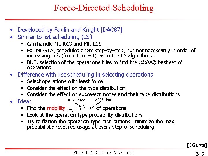
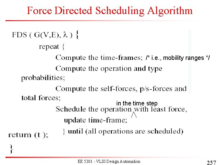
Force-Directed Scheduling • Developed by Paulin and Knight [DAC 87] • Similar to list scheduling (LS) § Can handle ML-RCS and MR-LCS § For ML-RCS, schedules opers step-by-step, but not necessarily in order of increasing cc’s (from 1 to last), as in the LS algorithms. § BUT, selection of the operations tries to find the globally best set of operations • Difference with list scheduling in selecting operations § Select operations with least force § Consider the effect on the type distribution § Consider the effect on successor nodes and their type distributions • Idea: ALAP time ASAP time § Find the mobility mi = ti. L – ti. S of operations § Look at the operation type probability distributions § Try to flatten the operation type distributions: minimize the max probabilistic resource usage at every step of scheduling [©Gupta] EE 5301 - VLSI Design Automation 245

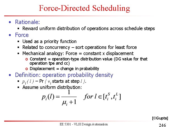
Force-Directed Scheduling • Rationale: § Reward uniform distribution of operations across schedule steps • Force § Used as a priority function § Related to concurrency – sort operations for least force § Mechanical analogy: Force = constant x displacement o Constant = operation-type distribution value (DG value for that operation tpe and cc) o Displacement = change in probability • Definition: operation probability density § pi ( l ) = Pr { vi starts at step l }. § Assume uniform distribution: [©Gupta] EE 5301 - VLSI Design Automation 246

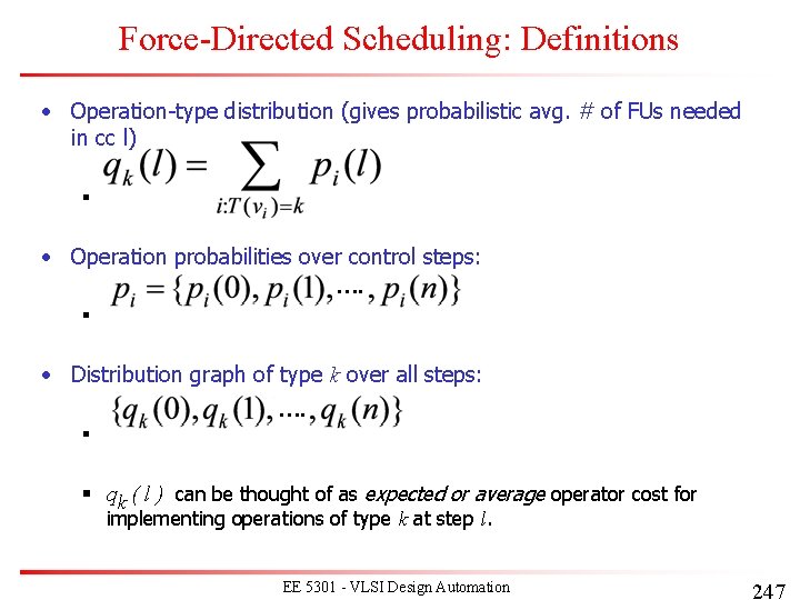
Force-Directed Scheduling: Definitions • Operation-type distribution (gives probabilistic avg. # of FUs needed in cc l) § • Operation probabilities over control steps: …. § • Distribution graph of type k over all steps: …. § § qk ( l ) can be thought of as expected or average operator cost for implementing operations of type k at step l. EE 5301 - VLSI Design Automation 247

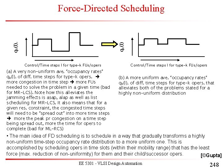
qk(l). Force-Directed Scheduling Control/Time steps l for type-k FUs/opers (a) A very non-uniform ave. “occupancy rates” qk(l). of diff. time steps for type-k opers. more congestion in time step more FUs needed to solve the problem in a given time (bad for MR-LCS). Note how this alleviates the jamming effects is asap, alap as well as list scheduling for MR-LCS. It also means that for a given res. constraint, the congested time steps will need to be “spread out” into more time steps more the peak pr congestion on a time step being spread out, more the time for opers to complete (bad for ML-RCS) Control/Time steps l for type-k FUs/opers (b) A more uniform ave. “occupancy rates” qk(l). of diff. time steps for type-k opers. that alleviates both of the problems stated for a highly non-uniform distribution • The main idea of FD scheduling is to schedule in a way that gradually transforms a highly non-uniform time-step occupancy rate distribution to a more uniform one. This is accomplished by scheduling opers in time slots (within their mobility range) that has the least force (max. reduction of non-uniformity) for them and their child/successor opers. [©Gupta] EE 5301 - VLSI Design Automation 248

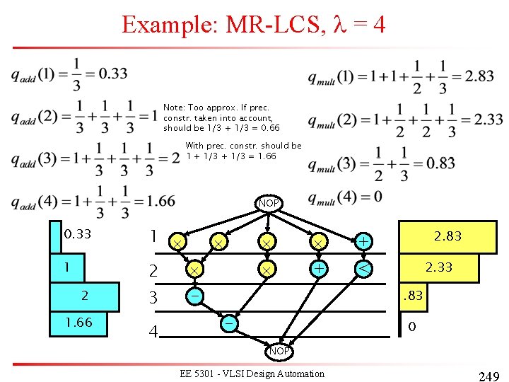
Example: MR-LCS, l = 4 Note: Too approx. If prec. constr. taken into account, should be 1/3 + 1/3 = 0. 66 With prec. constr. should be 1 + 1/3 = 1. 66 NOP 0. 33 1 1 2 2 1. 66 3 4 - + 2. 83 + < 2. 33. 83 - 0 NOP EE 5301 - VLSI Design Automation 249

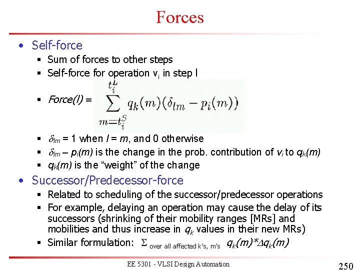
Forces • Self-force § Sum of forces to other steps § Self-force for operation vi in step l § Force(l) = § dlm = 1 when l = m, and 0 otherwise § dlm – pi(m) is the change in the prob. contribution of vi to qk(m) § qk(m) is the “weight” of the change • Successor/Predecessor-force § Related to scheduling of the successor/predecessor operations § For example, delaying an operation may cause the delay of its successors (shrinking of their mobility ranges [MRs] and mobilities and thus increase in qk values in their new MRs) § Similar formulation: S over all affected k’s, m’s qk(m)*Dqk(m) EE 5301 - VLSI Design Automation 250

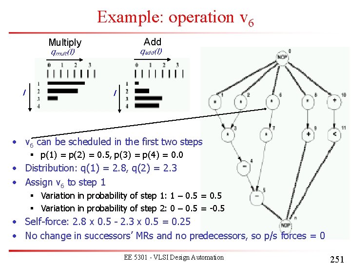
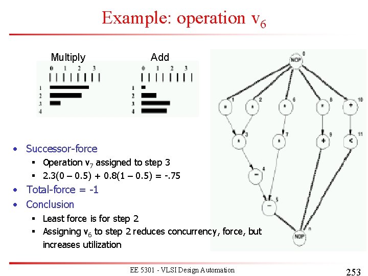
Example: operation v 6 Add Multiply qadd(l) qmult(l) l l • v 6 can be scheduled in the first two steps § p(1) = p(2) = 0. 5, p(3) = p(4) = 0. 0 • Distribution: q(1) = 2. 8, q(2) = 2. 3 • Assign v 6 to step 1 § Variation in probability of step 1: 1 – 0. 5 = 0. 5 § Variation in probability of step 2: 0 – 0. 5 = -0. 5 • Self-force: 2. 8 x 0. 5 - 2. 3 x 0. 5 = 0. 25 • No change in successors’ MRs and no predecessors, so p/s forces = 0 EE 5301 - VLSI Design Automation 251

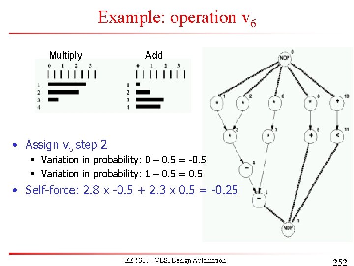
Example: operation v 6 Multiply Add • Assign v 6 step 2 § Variation in probability: 0 – 0. 5 = -0. 5 § Variation in probability: 1 – 0. 5 = 0. 5 • Self-force: 2. 8 x -0. 5 + 2. 3 x 0. 5 = -0. 25 EE 5301 - VLSI Design Automation 252

Example: operation v 6 Multiply Add • Successor-force § Operation v 7 assigned to step 3 § 2. 3(0 – 0. 5) + 0. 8(1 – 0. 5) = -. 75 • Total-force = -1 • Conclusion § Least force is for step 2 § Assigning v 6 to step 2 reduces concurrency, force, but increases utilization EE 5301 - VLSI Design Automation 253

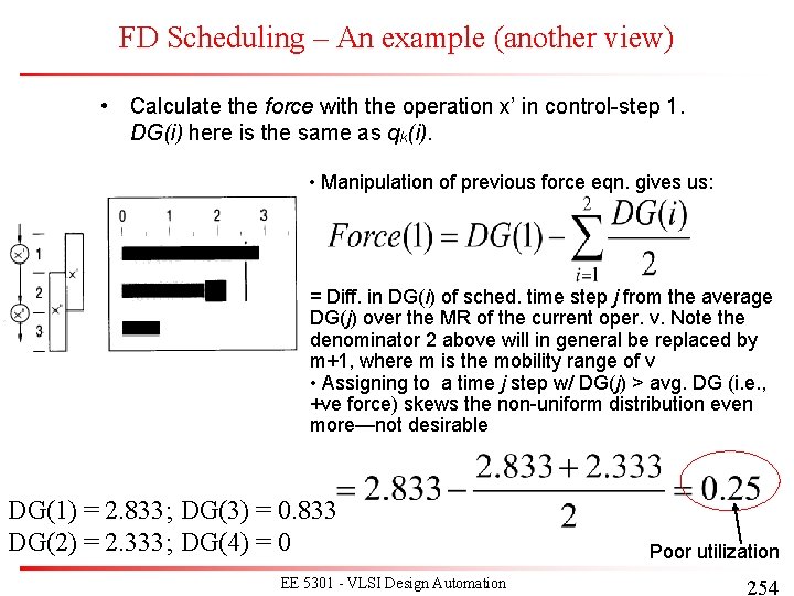
FD Scheduling – An example (another view) • Calculate the force with the operation x’ in control-step 1. DG(i) here is the same as qk(i). • Manipulation of previous force eqn. gives us: = Diff. in DG(i) of sched. time step j from the average DG(j) over the MR of the current oper. v. Note the denominator 2 above will in general be replaced by m+1, where m is the mobility range of v • Assigning to a time j step w/ DG(j) > avg. DG (i. e. , +ve force) skews the non-uniform distribution even more—not desirable DG(1) = 2. 833; DG(3) = 0. 833 DG(2) = 2. 333; DG(4) = 0 EE 5301 - VLSI Design Automation Poor utilization 254

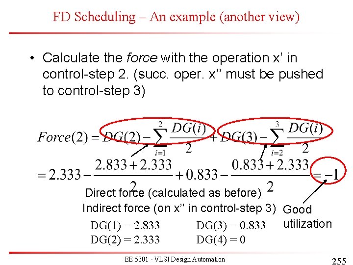
FD Scheduling – An example (another view) • Calculate the force with the operation x’ in control-step 2. (succ. oper. x’’ must be pushed to control-step 3) Direct force (calculated as before) Indirect force (on x’’ in control-step 3) Good DG(1) = 2. 833 DG(3) = 0. 833 utilization DG(2) = 2. 333 DG(4) = 0 EE 5301 - VLSI Design Automation 255

FD Scheduling • By repeatedly assigning operations to various control-steps and calculating the force associated with the choice, several force values will be available. • The Force-directed scheduling algorithm chooses the assignment with the lowest force value, which also balances the concurrency of operations most efficiently. EE 5301 - VLSI Design Automation 256

Force Directed Scheduling Algorithm /* i. e. , mobility ranges */ in the time step EE 5301 - VLSI Design Automation 257

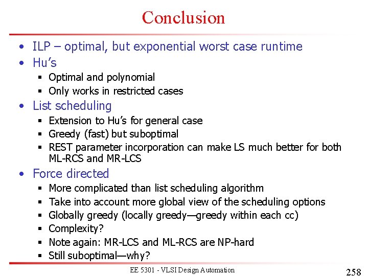
Conclusion • ILP – optimal, but exponential worst case runtime • Hu’s § Optimal and polynomial § Only works in restricted cases • List scheduling § Extension to Hu’s for general case § Greedy (fast) but suboptimal § REST parameter incorporation can make LS much better for both ML-RCS and MR-LCS • Force directed § § § More complicated than list scheduling algorithm Take into account more global view of the scheduling options Globally greedy (locally greedy—greedy within each cc) Complexity? Note again: MR-LCS and ML-RCS are NP-hard Still suboptimal—why? EE 5301 - VLSI Design Automation 258

To Probe Further. . . • Linear programming § http: //www. cs. sunysb. edu/~algorith/files/linearprogramming. shtml • Linear programming tools § http: //www-unix. mcs. anl. gov/otc/Guide/faq/linear-programmingfaq. html • Automatic compilation of pipelined designs § T. Maruyama and T. Hoshino, “A C to HDL Compiler for Pipeline Processing on FPGAs”, IEEE Symposium on FPGAs for Custom Computing Machines (FCCM), pp. 101 -110, 2001. EE 5301 - VLSI Design Automation 259