ECE 546 Lecture 22 Timing Signaling Spring 2016

ECE 546 Lecture - 22 Timing & Signaling Spring 2016 Jose E. Schutt-Aine Electrical & Computer Engineering University of Illinois jesa@illinois. edu ECE 546 – Jose Schutt-Aine 1

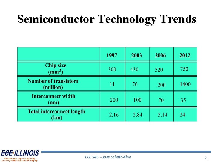
Semiconductor Technology Trends ECE 546 – Jose Schutt-Aine 2

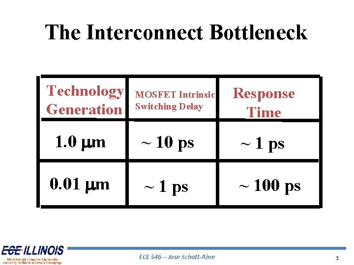
The Interconnect Bottleneck Technology Generation MOSFET Intrinsic Switching Delay Response Time 1. 0 mm ~ 10 ps ~ 1 ps 0. 01 mm ~ 1 ps ~ 100 ps ECE 546 – Jose Schutt-Aine 3

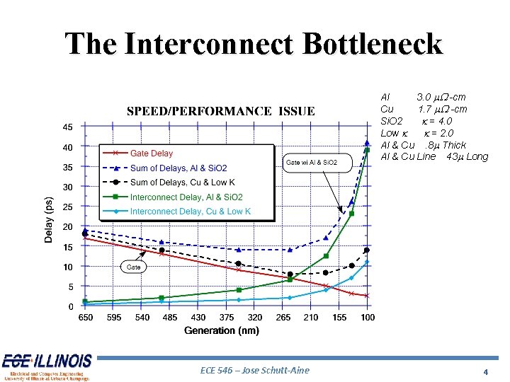
The Interconnect Bottleneck Al 3. 0 m. W -cm Cu 1. 7 m. W -cm Si. O 2 k = 4. 0 Low k k = 2. 0 Al & Cu. 8 m Thick Al & Cu Line 43 m Long ECE 546 – Jose Schutt-Aine 4

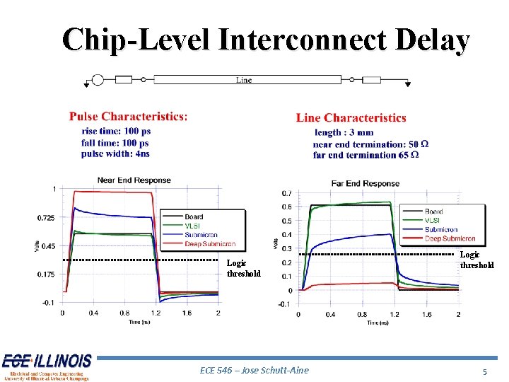
Chip-Level Interconnect Delay Logic threshold ECE 546 – Jose Schutt-Aine Logic threshold 5

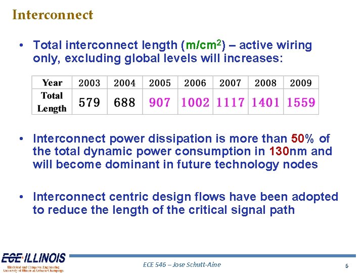
Interconnect • Total interconnect length (m/cm 2) – active wiring only, excluding global levels will increases: • Interconnect power dissipation is more than 50% of the total dynamic power consumption in 130 nm and will become dominant in future technology nodes • Interconnect centric design flows have been adopted to reduce the length of the critical signal path ECE 546 – Jose Schutt-Aine 6

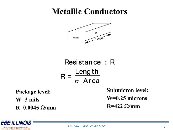
ECE 546 – Jose Schutt-Aine 7

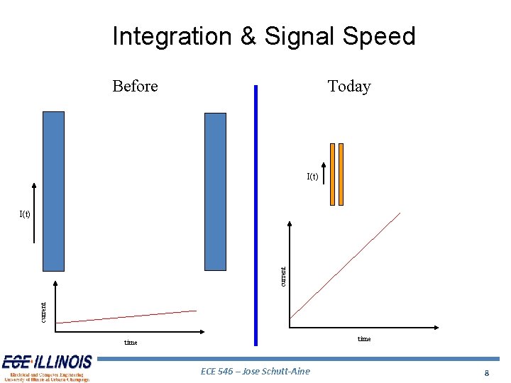
Integration & Signal Speed Before Today I(t) current I(t) time ECE 546 – Jose Schutt-Aine 8

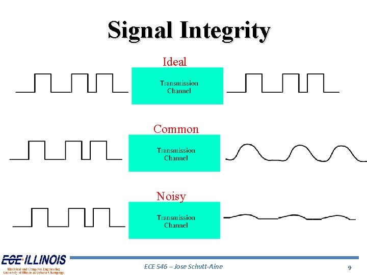
Signal Integrity Ideal Common Noisy ECE 546 – Jose Schutt-Aine 9

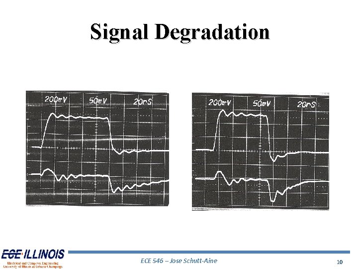
Signal Degradation ECE 546 – Jose Schutt-Aine 10

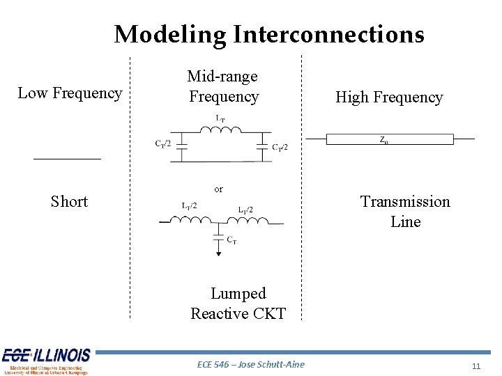
Modeling Interconnections Low Frequency Short Mid-range Frequency or High Frequency Transmission Line Lumped Reactive CKT ECE 546 – Jose Schutt-Aine 11

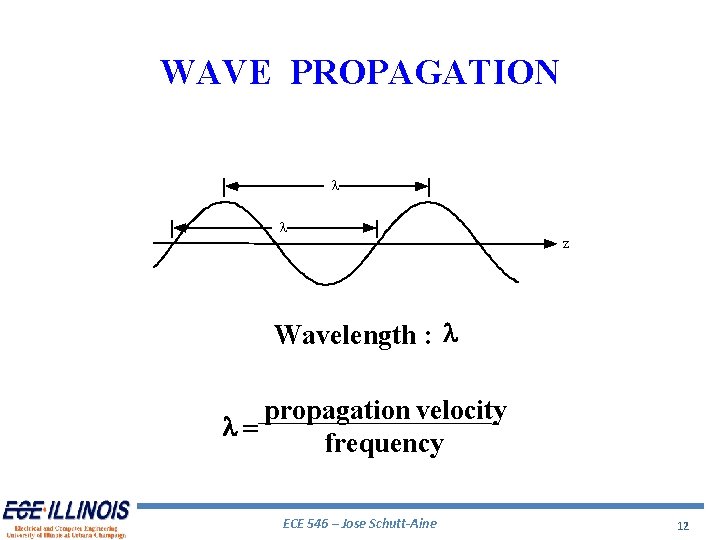
WAVE PROPAGATION l l z Wavelength : l propagation velocity l= frequency ECE 546 – Jose Schutt-Aine 12

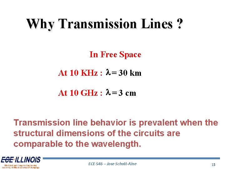
Why Transmission Lines ? In Free Space At 10 KHz : l = 30 km At 10 GHz : l = 3 cm Transmission line behavior is prevalent when the structural dimensions of the circuits are comparable to the wavelength. ECE 546 – Jose Schutt-Aine 13

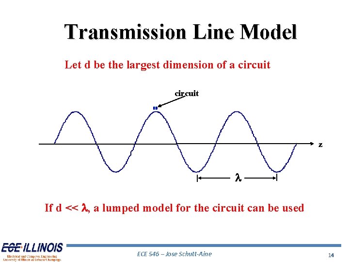
Transmission Line Model Let d be the largest dimension of a circuit z l If d << l, a lumped model for the circuit can be used ECE 546 – Jose Schutt-Aine 14

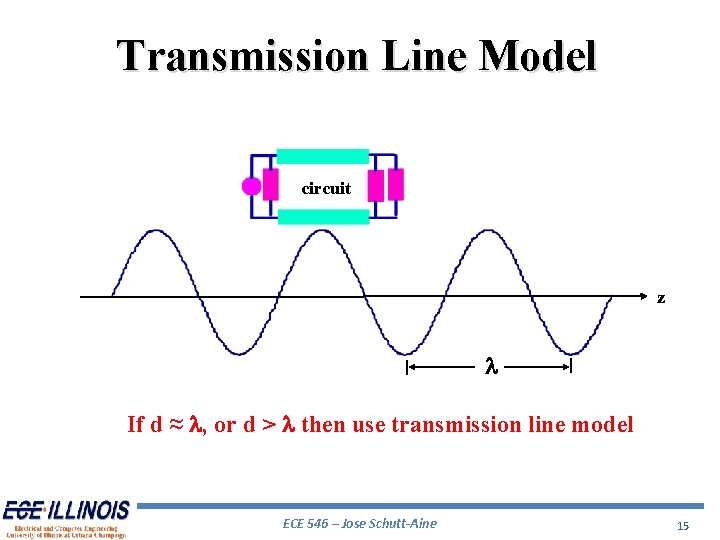
Transmission Line Model circuit z l If d ≈ l, or d > l then use transmission line model ECE 546 – Jose Schutt-Aine 15

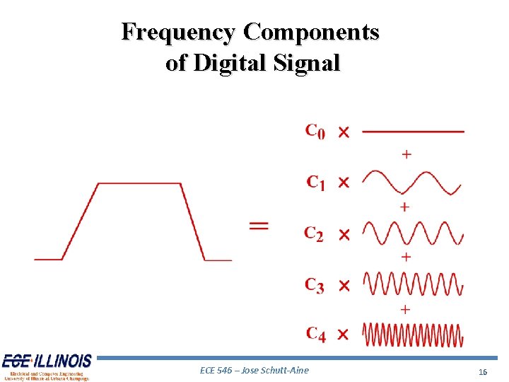
Frequency Components of Digital Signal ECE 546 – Jose Schutt-Aine 16

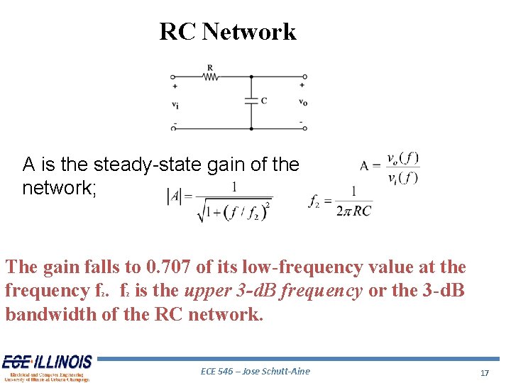
RC Network A is the steady-state gain of the network; The gain falls to 0. 707 of its low-frequency value at the frequency f. f is the upper 3 -d. B frequency or the 3 -d. B bandwidth of the RC network. 2 2 ECE 546 – Jose Schutt-Aine 17

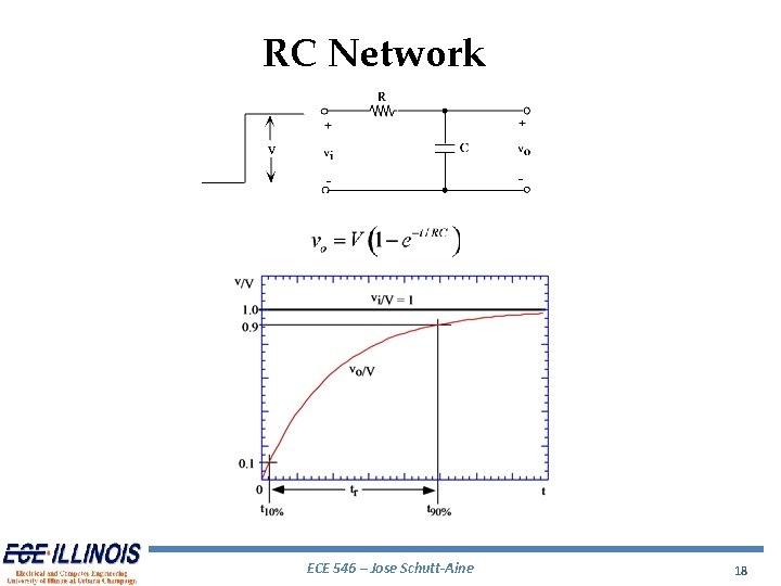
RC Network ECE 546 – Jose Schutt-Aine 18

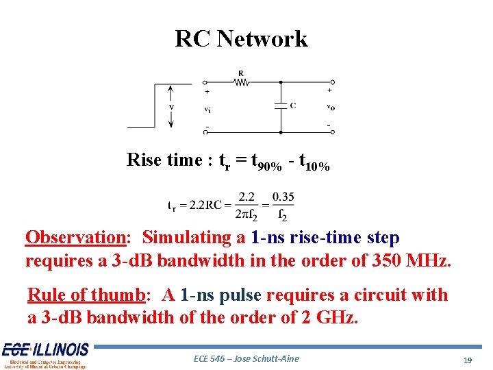
RC Network Rise time : tr = t 90% - t 10% Observation: Simulating a 1 -ns rise-time step requires a 3 -d. B bandwidth in the order of 350 MHz. Rule of thumb: A 1 -ns pulse requires a circuit with a 3 -d. B bandwidth of the order of 2 GHz. ECE 546 – Jose Schutt-Aine 19

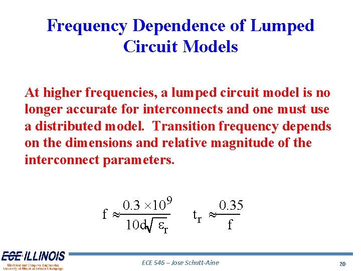
Frequency Dependence of Lumped Circuit Models At higher frequencies, a lumped circuit model is no longer accurate for interconnects and one must use a distributed model. Transition frequency depends on the dimensions and relative magnitude of the interconnect parameters. 0. 3 ´ 109 f » 10 d er 0. 35 tr » f ECE 546 – Jose Schutt-Aine 20

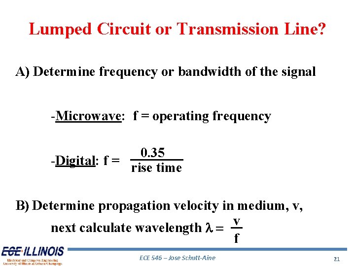
Lumped Circuit or Transmission Line? A) Determine frequency or bandwidth of the signal -Microwave: f = operating frequency 0. 35 -Digital: f = rise time B) Determine propagation velocity in medium, v, v next calculate wavelength l = f ECE 546 – Jose Schutt-Aine 21

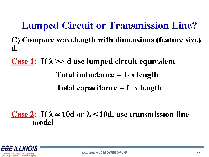
Lumped Circuit or Transmission Line? C) Compare wavelength with dimensions (feature size) d. Case 1: If l >> d use lumped circuit equivalent Total inductance = L x length Total capacitance = C x length Case 2: If l » 10 d or l < 10 d, use transmission-line model ECE 546 – Jose Schutt-Aine 22

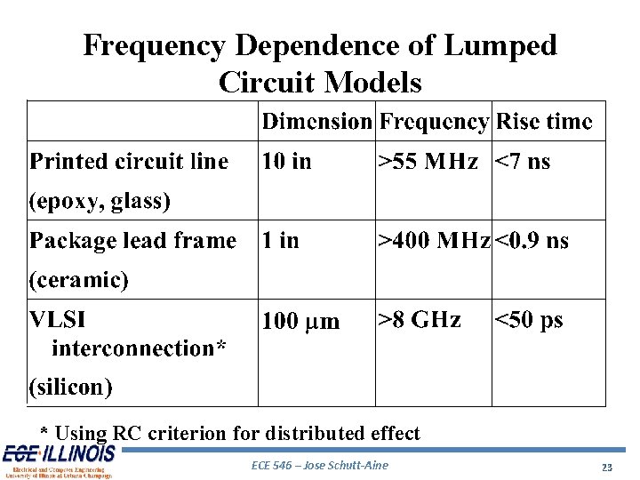
Frequency Dependence of Lumped Circuit Models * Using RC criterion for distributed effect ECE 546 – Jose Schutt-Aine 23

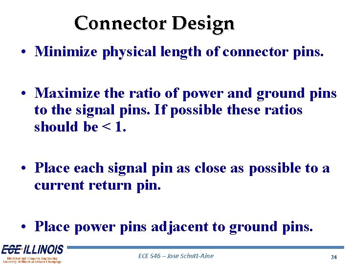
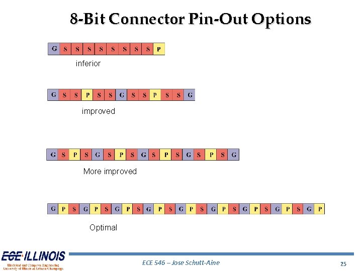
Connector Design • Minimize physical length of connector pins. • Maximize the ratio of power and ground pins to the signal pins. If possible these ratios should be < 1. • Place each signal pin as close as possible to a current return pin. • Place power pins adjacent to ground pins. ECE 546 – Jose Schutt-Aine 24

8 -Bit Connector Pin-Out Options inferior improved More improved Optimal ECE 546 – Jose Schutt-Aine 25

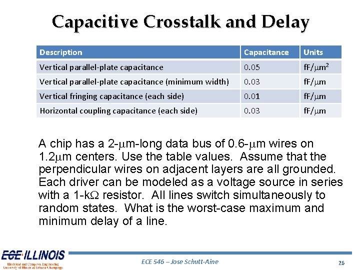
Capacitive Crosstalk and Delay Description Capacitance Units Vertical parallel-plate capacitance 0. 05 f. F/mm 2 Vertical parallel-plate capacitance (minimum width) 0. 03 f. F/mm Vertical fringing capacitance (each side) 0. 01 f. F/mm Horizontal coupling capacitance (each side) 0. 03 f. F/mm A chip has a 2 -mm-long data bus of 0. 6 -mm wires on 1. 2 mm centers. Use the table values. Assume that the perpendicular wires on adjacent layers are all grounded. Each driver can be modeled as a voltage source in series with a 1 -k. W resistor. All lines switch simultaneously to random states. What is the worst-case maximum and minimum delay of a line. ECE 546 – Jose Schutt-Aine 26

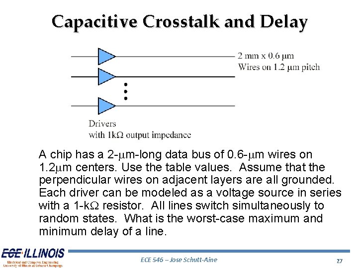
Capacitive Crosstalk and Delay A chip has a 2 -mm-long data bus of 0. 6 -mm wires on 1. 2 mm centers. Use the table values. Assume that the perpendicular wires on adjacent layers are all grounded. Each driver can be modeled as a voltage source in series with a 1 -k. W resistor. All lines switch simultaneously to random states. What is the worst-case maximum and minimum delay of a line. ECE 546 – Jose Schutt-Aine 27

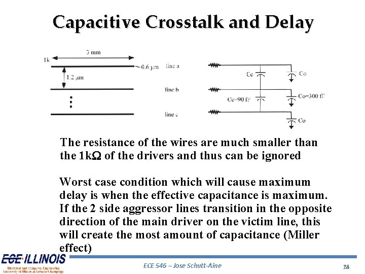
Capacitive Crosstalk and Delay The resistance of the wires are much smaller than the 1 k. W of the drivers and thus can be ignored Worst case condition which will cause maximum delay is when the effective capacitance is maximum. If the 2 side aggressor lines transition in the opposite direction of the main driver on the victim line, this will create the most amount of capacitance (Miller effect) ECE 546 – Jose Schutt-Aine 28

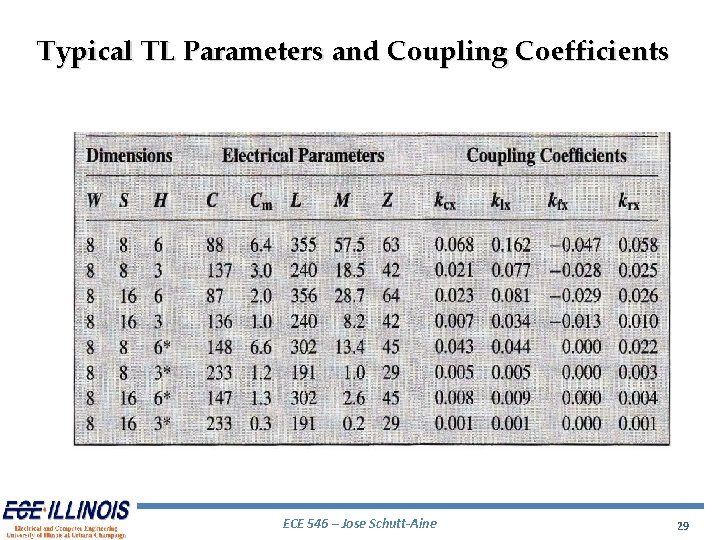
Typical TL Parameters and Coupling Coefficients ECE 546 – Jose Schutt-Aine 29

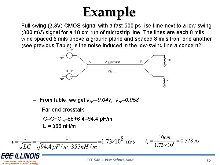
Example Full-swing (3. 3 V) CMOS signal with a fast 500 ps rise time next to a low-swing (300 m. V) signal for a 10 cm run of microstrip line. The lines are each 8 mils wide spaced 6 mils above a ground plane and spaced 8 mils from one another (see previous Table). Is the noise induced in the low-swing line a concern? – From table, we get kfx=-0. 047, krx=0. 058 Far end crosstalk C=C+Cm=88+6. 4=94. 4 p. F/m L = 355 n. H/m ECE 546 – Jose Schutt-Aine 30

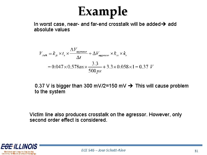
Example In worst case, near- and far-end crosstalk will be added add absolute values 0. 37 V is bigger than 300 m. V/2=150 m. V This will cause problem to the system Victim line also produces crosstalk on the agressor. However, only second order effect is considered. ECE 546 – Jose Schutt-Aine 31

Signaling Conventions • A good signaling convention isolates a signal from noise to provide noise immunity. • Most signaling conventions in common use are based on standards and are actually quite poor. • Many modern systems define their own signaling conventions rather than employ the standards ECE 546 – Jose Schutt-Aine 32

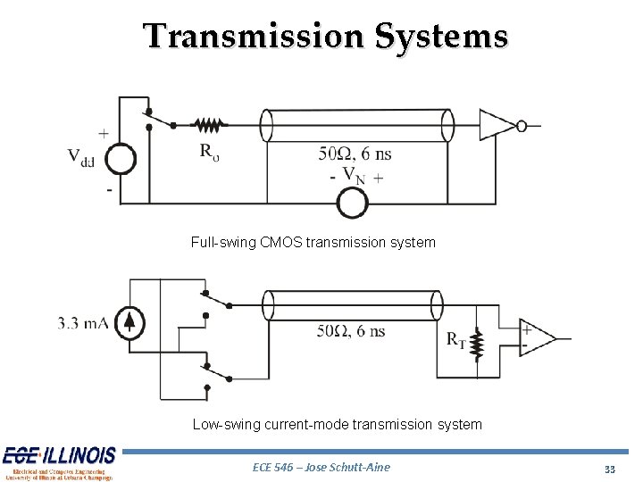
Transmission Systems Full-swing CMOS transmission system Low-swing current-mode transmission system ECE 546 – Jose Schutt-Aine 33

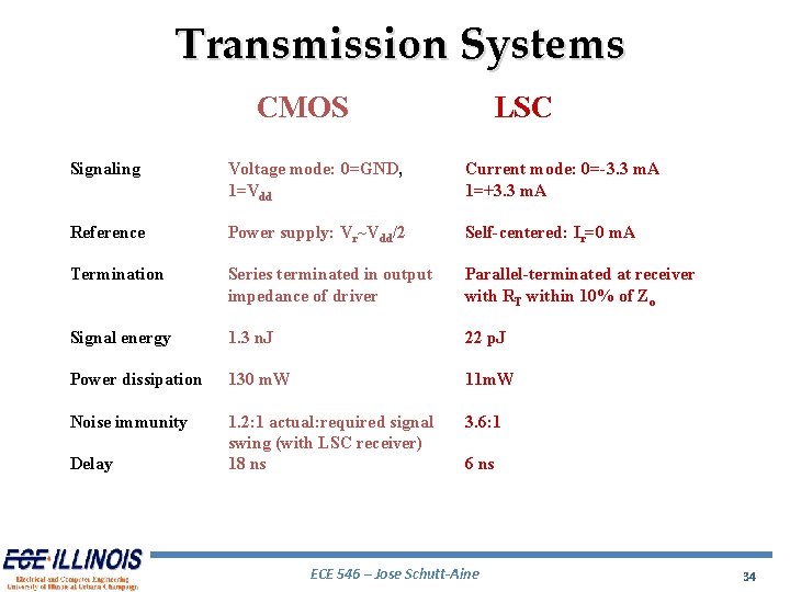
Transmission Systems CMOS LSC Signaling Voltage mode: 0=GND, 1=Vdd Current mode: 0=-3. 3 m. A 1=+3. 3 m. A Reference Power supply: Vr~Vdd/2 Self-centered: Ir=0 m. A Termination Series terminated in output impedance of driver Parallel-terminated at receiver with RT within 10% of Zo Signal energy 1. 3 n. J 22 p. J Power dissipation 130 m. W 11 m. W Noise immunity 1. 2: 1 actual: required signal swing (with LSC receiver) 18 ns 3. 6: 1 Delay 6 ns ECE 546 – Jose Schutt-Aine 34

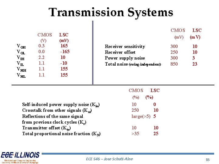
Transmission Systems VOH VOL VIH VIL VMH VML CMOS LSC (V) (m. V) 0. 3 0. 0 2. 2 1. 1 CMOS (m. V) 165 -165 10 -10 155 Receiver sensitivity Receiver offset Power supply noise Total noise (swing-independent) CMOS (%) Self-induced power supply noise (Kin) Crosstalk from other signals (Kxt) Reflections of the same signal from previous clock cycles (Kr) Transmitter offset (Kto) Total proportional noise fraction (KN) 300 250 300 850 LSC (m. V) 10 10 3 23 LSC (%) 10 0 250 10 large(>5) 5 10 >35 ECE 546 – Jose Schutt-Aine 10 25 35

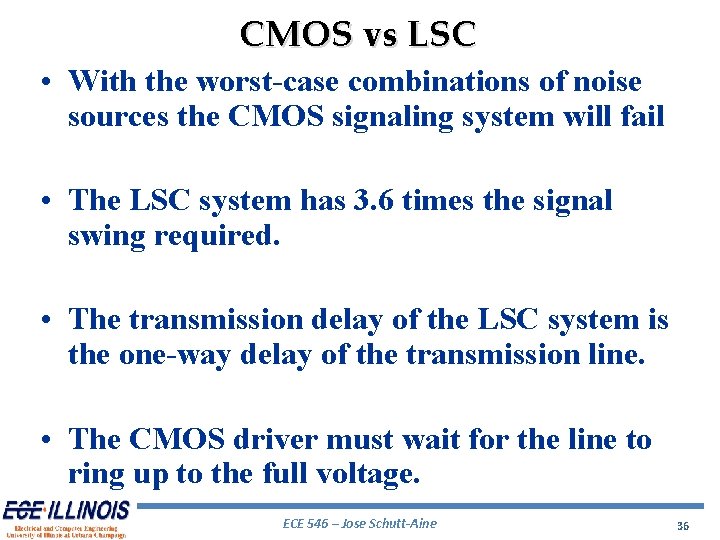
CMOS vs LSC • With the worst-case combinations of noise sources the CMOS signaling system will fail • The LSC system has 3. 6 times the signal swing required. • The transmission delay of the LSC system is the one-way delay of the transmission line. • The CMOS driver must wait for the line to ring up to the full voltage. ECE 546 – Jose Schutt-Aine 36

CMOS vs LSC • Basic CMOS system is most commonly used and yet is far from optimal • Large energy signal is used where it is not needed • Transmitted signal not isolated from supply noise • Receiver uses reference that changes significantly with process variations ECE 546 – Jose Schutt-Aine 37

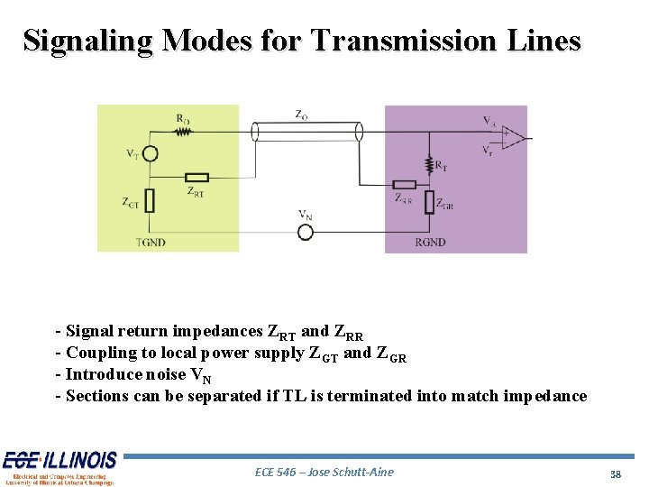
Signaling Modes for Transmission Lines - Signal return impedances ZRT and ZRR - Coupling to local power supply ZGT and ZGR - Introduce noise VN - Sections can be separated if TL is terminated into match impedance ECE 546 – Jose Schutt-Aine 38

Transmitter Signaling Parameters • Output impedance, Ro • Coupling between signal and power supply ZGT • Polarity of signal • Amplitude of signal ECE 546 – Jose Schutt-Aine 39

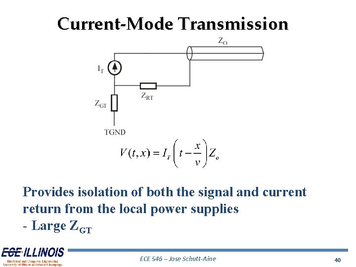
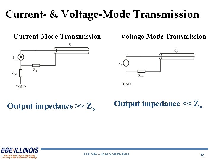
Current-Mode Transmission Provides isolation of both the signal and current return from the local power supplies - Large ZGT ECE 546 – Jose Schutt-Aine 40

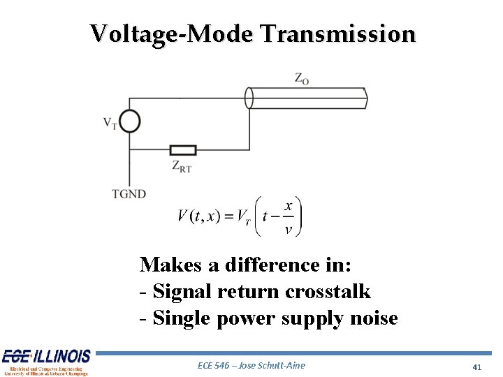
Voltage-Mode Transmission Makes a difference in: - Signal return crosstalk - Single power supply noise ECE 546 – Jose Schutt-Aine 41

Current- & Voltage-Mode Transmission Current-Mode Transmission Output impedance >> Zo Voltage-Mode Transmission Output impedance << Zo ECE 546 – Jose Schutt-Aine 42

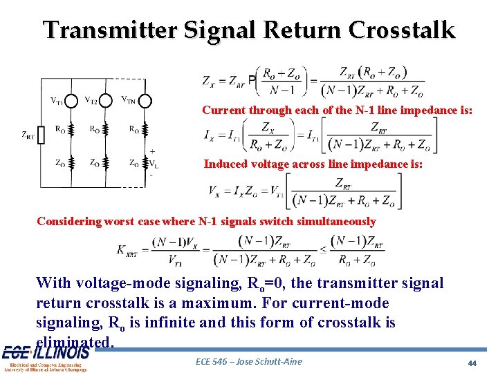
Transmitter Signal-Return Crosstalk • A signal return path is typically shared among a group of N signals (typically 2 to 8) to reduce cost. • Sharing occurs at both ends of line. • ZRT approximates the return path impedance at the transmitter end. • The return current from all N transmission lines passes through impedance ZRT. • The current IT 1 = VT 1/Zo sees the shared return impedance in parallel with the series combination of the line and output impedances from other signals. • The total return impedance is ZX. ECE 546 – Jose Schutt-Aine 43

Transmitter Signal Return Crosstalk Current through each of the N-1 line impedance is: Induced voltage across line impedance is: Considering worst case where N-1 signals switch simultaneously With voltage-mode signaling, Ro=0, the transmitter signal return crosstalk is a maximum. For current-mode signaling, Ro is infinite and this form of crosstalk is eliminated. ECE 546 – Jose Schutt-Aine 44

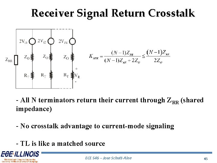
Receiver Signal Return Crosstalk - All N terminators return their current through ZRR (shared impedance) - No crosstalk advantage to current-mode signaling - TL is like a matched source ECE 546 – Jose Schutt-Aine 45

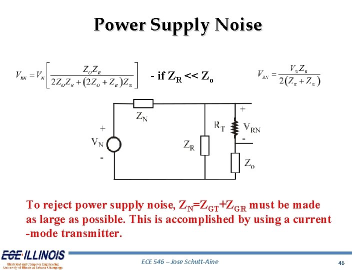
Power Supply Noise - if ZR << Zo To reject power supply noise, ZN=ZGT+ZGR must be made as large as possible. This is accomplished by using a current -mode transmitter. ECE 546 – Jose Schutt-Aine 46

Nonideal Return Paths • A nonideal return path will appear as an inductive discontinuity • A nonideal return path will slow the edge rate by filtering out high-frequency components • If the current divergence path is long enough, a nonideal return path will cause signal integrity problems at the receiver • Nonideal return paths will increase current loop area and exacerbate EMI • Nonideal return paths may significantly increase the coupling coefficient between signals ECE 546 – Jose Schutt-Aine 47

Signal Return Crosstalk • Return crosstalk can be reduced with rise-time control • As rise times get faster, every signal requires its own return might as well use differential signaling • With voltage-mode signaling, the transmitter signal return crosstalk is a maximum • High output impedance offers advantage and reduces transmitter return crosstalk • For current-mode signaling, this form of crosstalk is completely eliminated ECE 546 – Jose Schutt-Aine 48

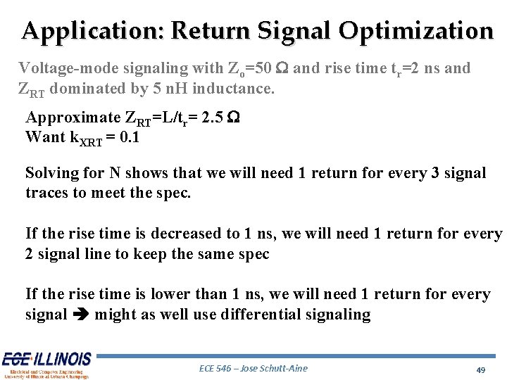
Application: Return Signal Optimization Voltage-mode signaling with Zo=50 W and rise time tr=2 ns and ZRT dominated by 5 n. H inductance. Approximate ZRT=L/tr= 2. 5 W Want k. XRT = 0. 1 Solving for N shows that we will need 1 return for every 3 signal traces to meet the spec. If the rise time is decreased to 1 ns, we will need 1 return for every 2 signal line to keep the same spec If the rise time is lower than 1 ns, we will need 1 return for every signal might as well use differential signaling ECE 546 – Jose Schutt-Aine 49

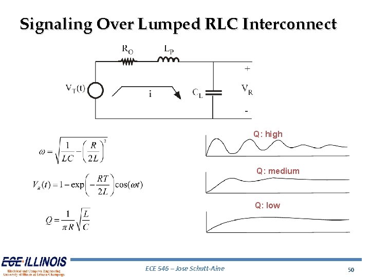
Signaling Over Lumped RLC Interconnect Q: high Q: medium Q: low ECE 546 – Jose Schutt-Aine 50

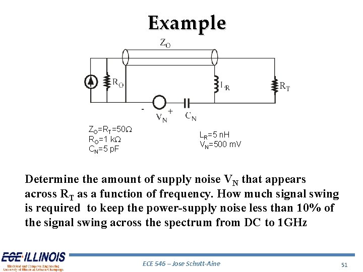
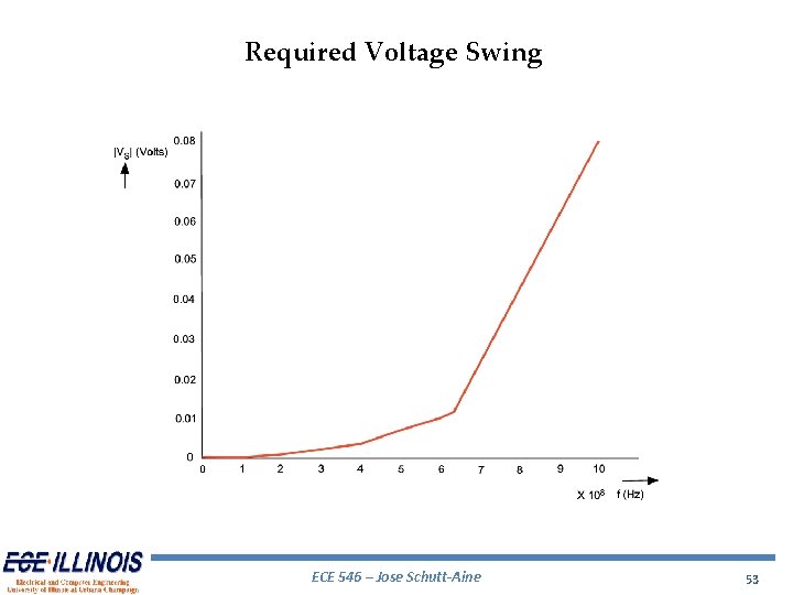
Example ZO=RT=50 W RO=1 k. W CN=5 p. F LR=5 n. H VN=500 m. V Determine the amount of supply noise VN that appears across RT as a function of frequency. How much signal swing is required to keep the power-supply noise less than 10% of the signal swing across the spectrum from DC to 1 GHz ECE 546 – Jose Schutt-Aine 51

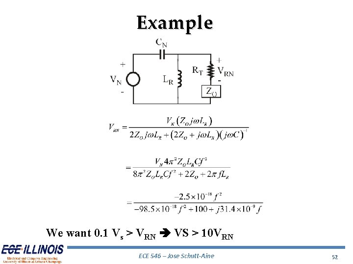
Example We want 0. 1 Vs > VRN VS > 10 VRN ECE 546 – Jose Schutt-Aine 52

Required Voltage Swing ECE 546 – Jose Schutt-Aine 53

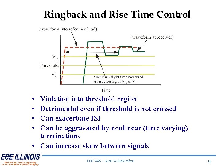
Ringback and Rise Time Control • • Violation into threshold region Detrimental even if threshold is not crossed Can exacerbate ISI Can be aggravated by nonlinear (time varying) terminations • Can increase skew between signals ECE 546 – Jose Schutt-Aine 54

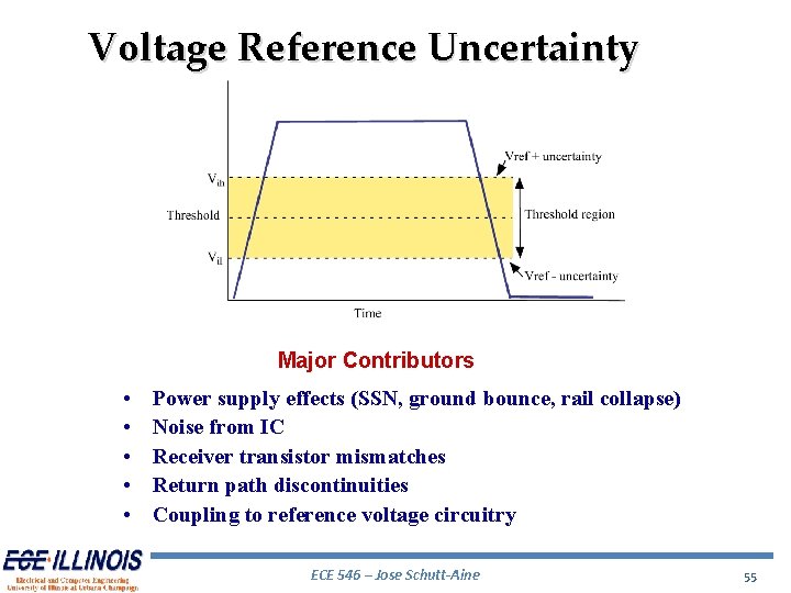
Voltage Reference Uncertainty Major Contributors • • • Power supply effects (SSN, ground bounce, rail collapse) Noise from IC Receiver transistor mismatches Return path discontinuities Coupling to reference voltage circuitry ECE 546 – Jose Schutt-Aine 55

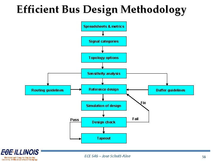
Efficient Bus Design Methodology Spreadsheets & metrics Signal categories Topology options Sensitivity analysis Reference design Routing guidelines Buffer guidelines Fix Simulation of design Pass Design check Fail Tapeout ECE 546 – Jose Schutt-Aine 56

Bus System Variables • • I/O capacitance Trace length, velocity, and impedance Interlayer impedance variations Buffer strengths and edge rates Termination values Receiver setup and hold times Interconnect skew specifications Package, daughtercard, and parameters ECE 546 – Jose Schutt-Aine 57

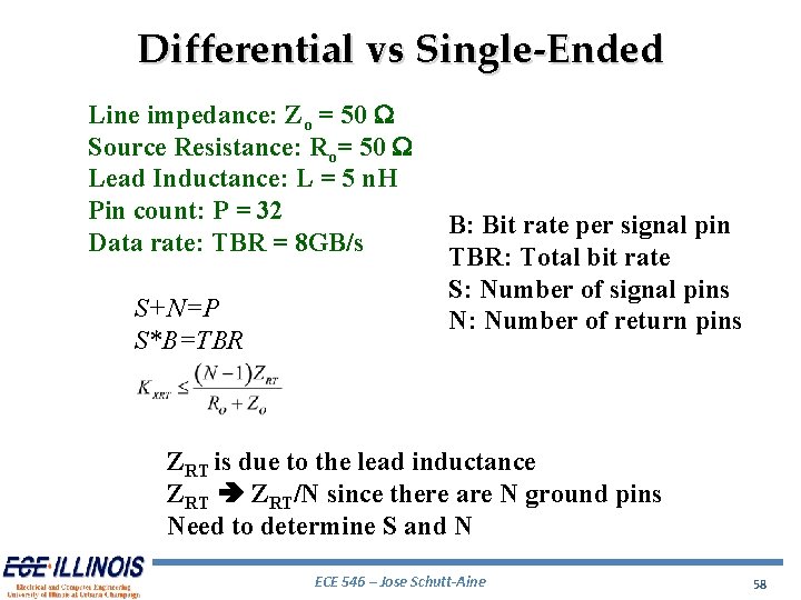
Differential vs Single-Ended Line impedance: Zo = 50 W Source Resistance: Ro= 50 W Lead Inductance: L = 5 n. H Pin count: P = 32 Data rate: TBR = 8 GB/s S+N=P S*B=TBR B: Bit rate per signal pin TBR: Total bit rate S: Number of signal pins N: Number of return pins ZRT is due to the lead inductance ZRT/N since there are N ground pins Need to determine S and N ECE 546 – Jose Schutt-Aine 58

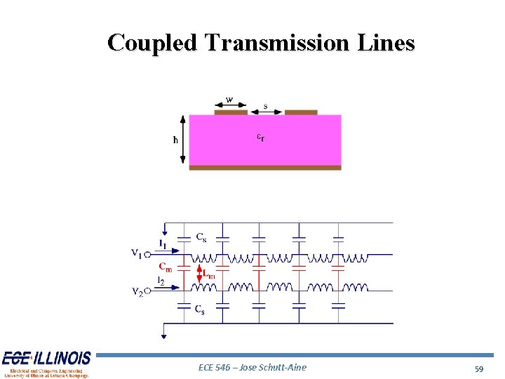
Coupled Transmission Lines ECE 546 – Jose Schutt-Aine 59

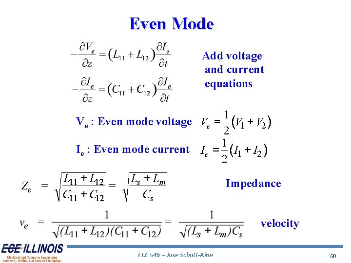
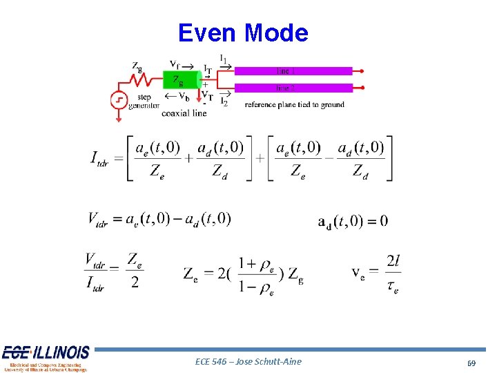
Even Mode Add voltage and current equations Ve : Even mode voltage Ie : Even mode current Impedance velocity ECE 546 – Jose Schutt-Aine 60

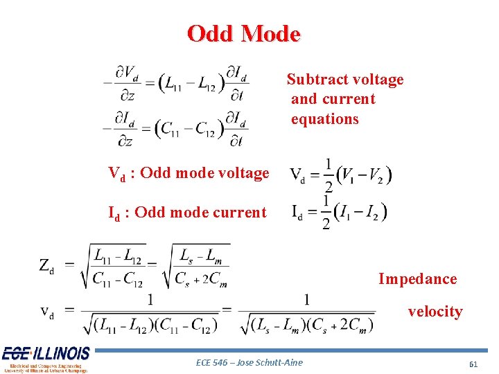
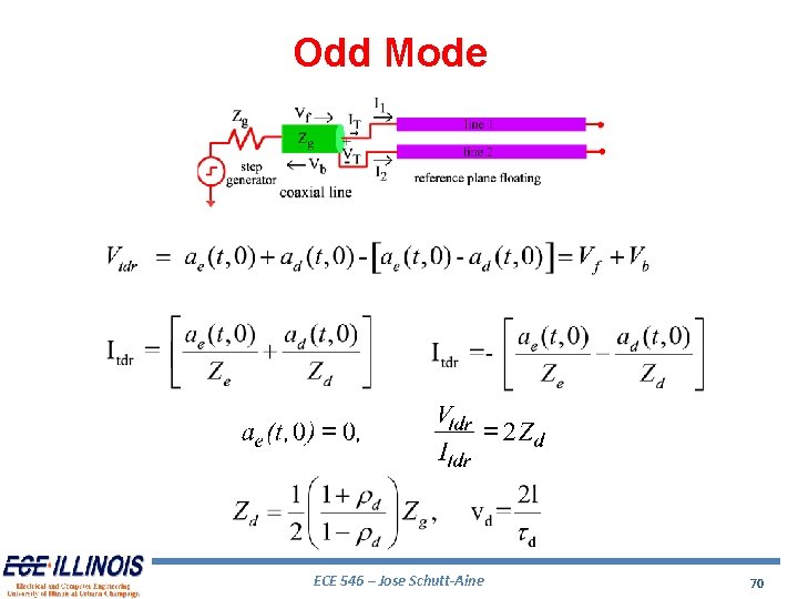
Odd Mode Subtract voltage and current equations Vd : Odd mode voltage Id : Odd mode current Impedance velocity ECE 546 – Jose Schutt-Aine 61

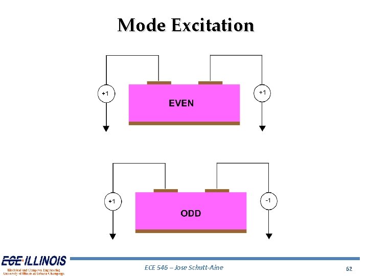
Mode Excitation ECE 546 – Jose Schutt-Aine 62

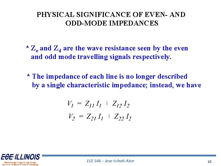
PHYSICAL SIGNIFICANCE OF EVEN- AND ODD-MODE IMPEDANCES * Ze and Zd are the wave resistance seen by the even and odd mode travelling signals respectively. * The impedance of each line is no longer described by a single characteristic impedance; instead, we have ECE 546 – Jose Schutt-Aine 63

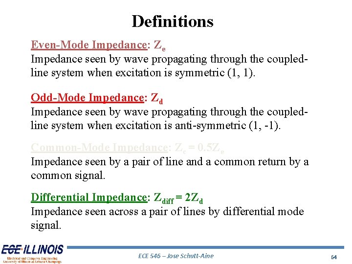
Definitions Even-Mode Impedance: Ze Impedance seen by wave propagating through the coupledline system when excitation is symmetric (1, 1). Odd-Mode Impedance: Zd Impedance seen by wave propagating through the coupledline system when excitation is anti-symmetric (1, -1). Common-Mode Impedance: Zc = 0. 5 Ze Impedance seen by a pair of line and a common return by a common signal. Differential Impedance: Zdiff = 2 Zd Impedance seen across a pair of lines by differential mode signal. ECE 546 – Jose Schutt-Aine 64

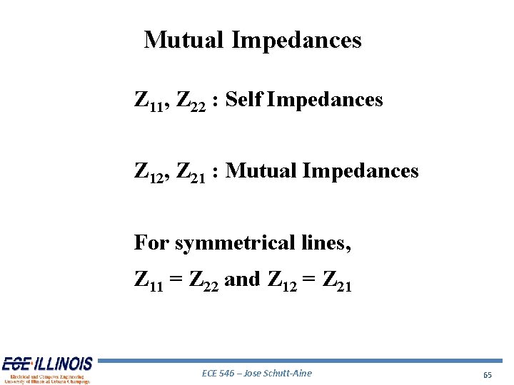
Mutual Impedances Z 11, Z 22 : Self Impedances Z 12, Z 21 : Mutual Impedances For symmetrical lines, Z 11 = Z 22 and Z 12 = Z 21 ECE 546 – Jose Schutt-Aine 65

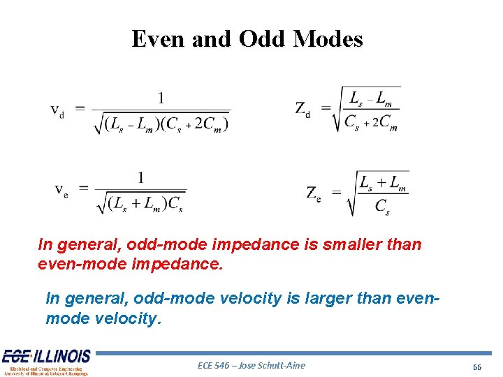
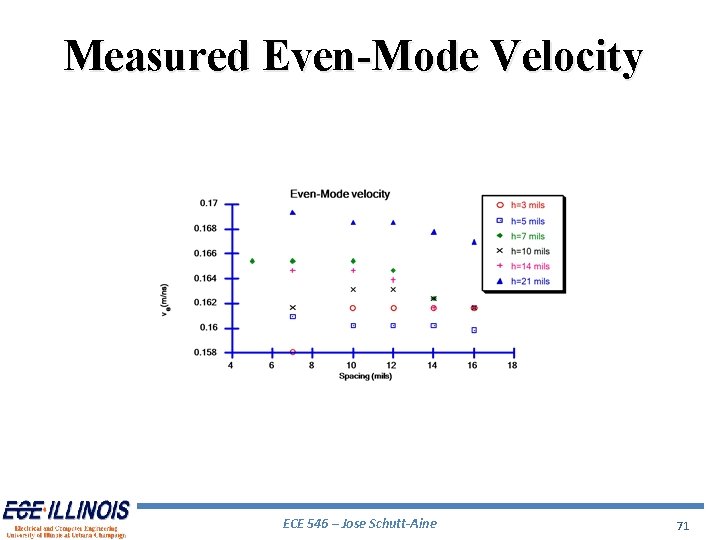
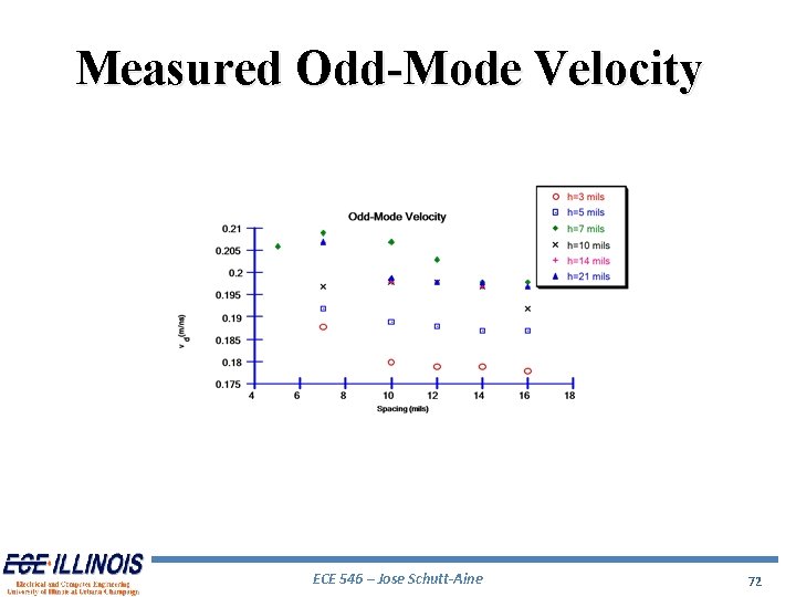
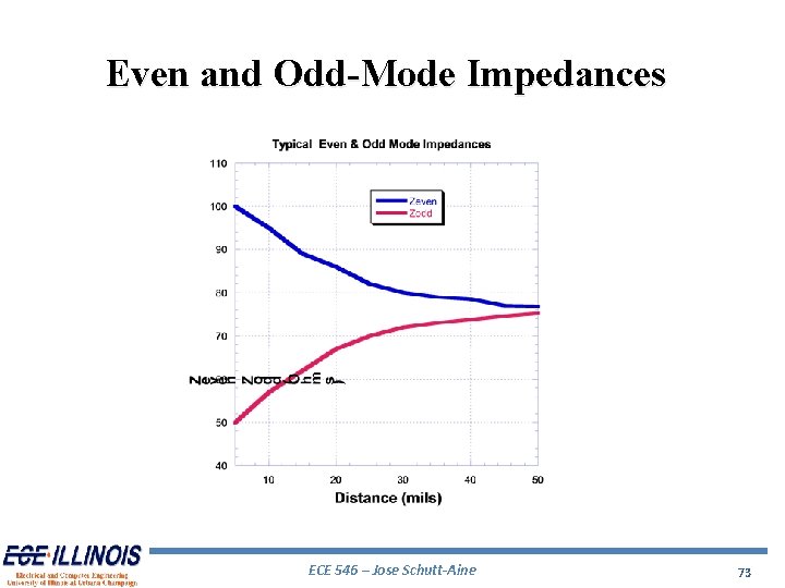
Even and Odd Modes In general, odd-mode impedance is smaller than even-mode impedance. In general, odd-mode velocity is larger than evenmode velocity. ECE 546 – Jose Schutt-Aine 66

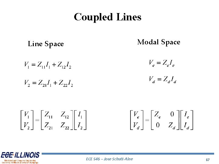
Coupled Lines Modal Space Line Space ECE 546 – Jose Schutt-Aine 67

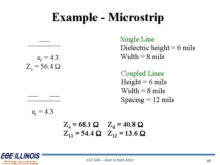
Example - Microstrip er = 4. 3 Zs = 56. 4 W Single Line Dielectric height = 6 mils Width = 8 mils Coupled Lines Height = 6 mils Width = 8 mils Spacing = 12 mils er = 4. 3 Ze = 68. 1 W Zd = 40. 8 W Z 11 = 54. 4 W Z 12 = 13. 6 W ECE 546 – Jose Schutt-Aine 68

Even Mode ECE 546 – Jose Schutt-Aine 69

Odd Mode ECE 546 – Jose Schutt-Aine 70

Measured Even-Mode Velocity ECE 546 – Jose Schutt-Aine 71

Measured Odd-Mode Velocity ECE 546 – Jose Schutt-Aine 72

Even and Odd-Mode Impedances ECE 546 – Jose Schutt-Aine 73

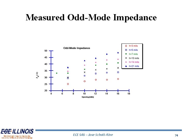
Measured Odd-Mode Impedance ECE 546 – Jose Schutt-Aine 74

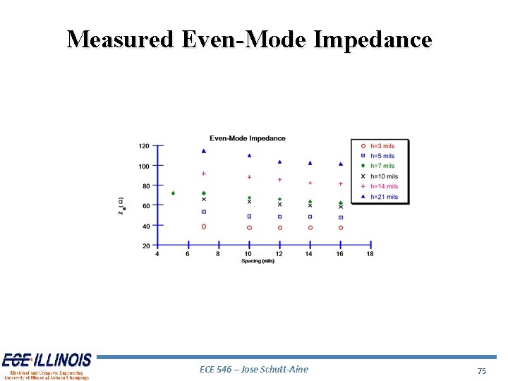
Measured Even-Mode Impedance ECE 546 – Jose Schutt-Aine 75

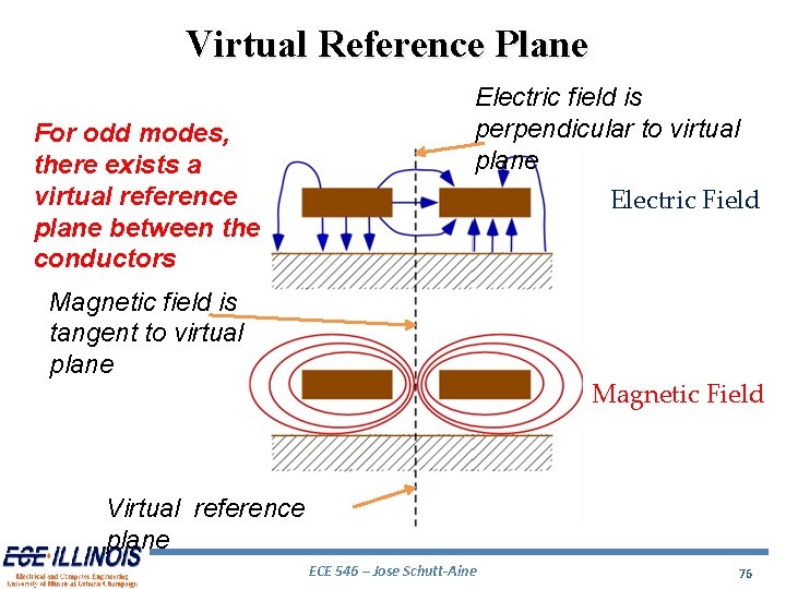
Virtual Reference Plane For odd modes, there exists a virtual reference plane between the conductors Electric field is perpendicular to virtual plane Electric Field Magnetic field is tangent to virtual plane Magnetic Field Virtual reference plane ECE 546 – Jose Schutt-Aine 76

Low-Voltage Differential Signaling (LVDS) Definition: Method to communicate data using a very low voltage swing (about 350 m. V) differentially over two PCB traces or a balanced cable Criteria for high-performance communication - Bandwidth - Low Power - Low Noise Solution exists for very short and very long distances; however for board-to-board or box-to-box, this is a challenge ECE 546 – Jose Schutt-Aine 77

Why LVDS? 1. Differential transmission is less susceptible to common mode noise 2. Consequently they can use lower voltage swings 3. In PC board (microstrip) odd-mode propagation is faster ECE 546 – Jose Schutt-Aine 78

LVDS Attributes for EMI 1. Low output voltage swing 2. Slow edge rates 3. Odd-mode operation (magnetic fields cancel) 4. Soft output corner transitions ECE 546 – Jose Schutt-Aine 79

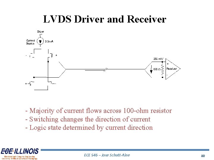
LVDS Driver and Receiver - Majority of current flows across 100 -ohm resistor - Switching changes the direction of current - Logic state determined by current direction ECE 546 – Jose Schutt-Aine 80

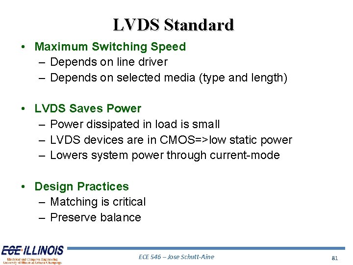
LVDS Standard • Maximum Switching Speed – Depends on line driver – Depends on selected media (type and length) • LVDS Saves Power – Power dissipated in load is small – LVDS devices are in CMOS=>low static power – Lowers system power through current-mode • Design Practices – Matching is critical – Preserve balance ECE 546 – Jose Schutt-Aine 81

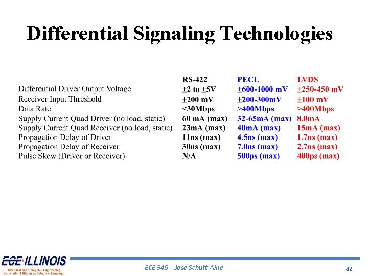
Differential Signaling Technologies ECE 546 – Jose Schutt-Aine 82