ECE 530 Analysis Techniques for LargeScale Electrical Systems

ECE 530 – Analysis Techniques for Large-Scale Electrical Systems Lecture 4: Newton-Raphson Power Flow Prof. Hao Zhu Dept. of Electrical and Computer Engineering University of Illinois at Urbana-Champaign haozhu@illinois. edu 9/2/2015 1

Announcements • • • No class next Monday (labor day) Homework 1 due next Wednesday, in class A reference book on linear algebra: The Matrix Cookbook http: //www. math. uwaterloo. ca/~hwolkowi/matrixcookb ook. pdf 2

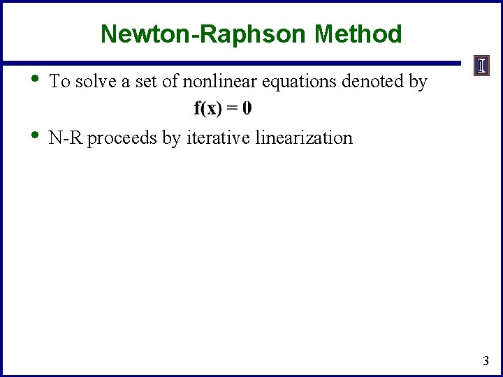
Newton-Raphson Method • To solve a set of nonlinear equations denoted by • N-R proceeds by iterative linearization 3

Power Flow Variables 4

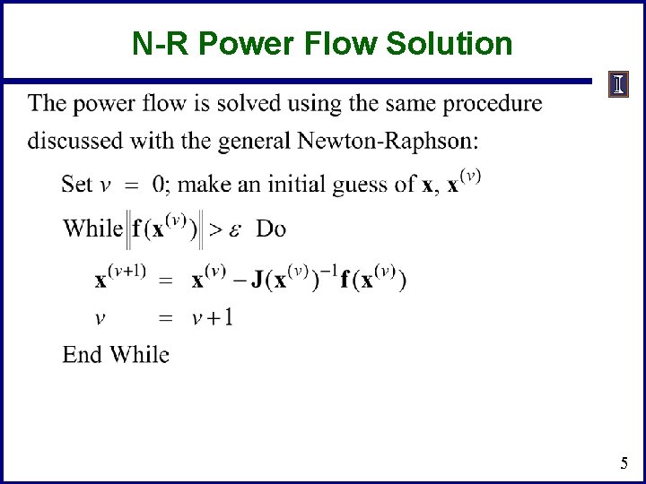
N-R Power Flow Solution 5

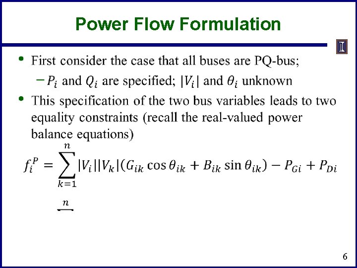
Power Flow Formulation 6

Jacobian Matrix 7

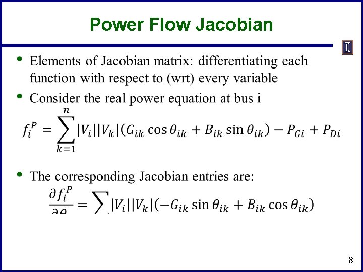
Power Flow Jacobian 8

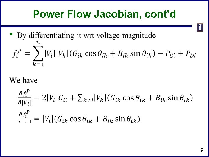
Power Flow Jacobian, cont’d 9

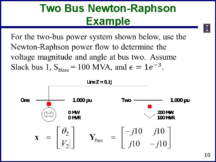
Two Bus Newton-Raphson Example 10

Two Bus Example, cont’d 11

Two Bus Example, cont’d 2 2 12

Two Bus Example, First Iteration 13

Two Bus Example, Convergence 14

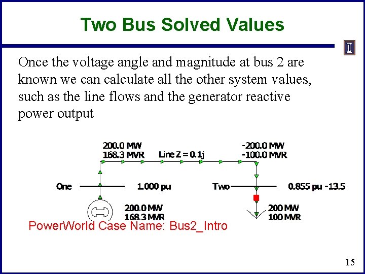
Two Bus Solved Values Once the voltage angle and magnitude at bus 2 are known we can calculate all the other system values, such as the line flows and the generator reactive power output Power. World Case Name: Bus 2_Intro 15

Two Bus Case, Low Voltage Solution 16

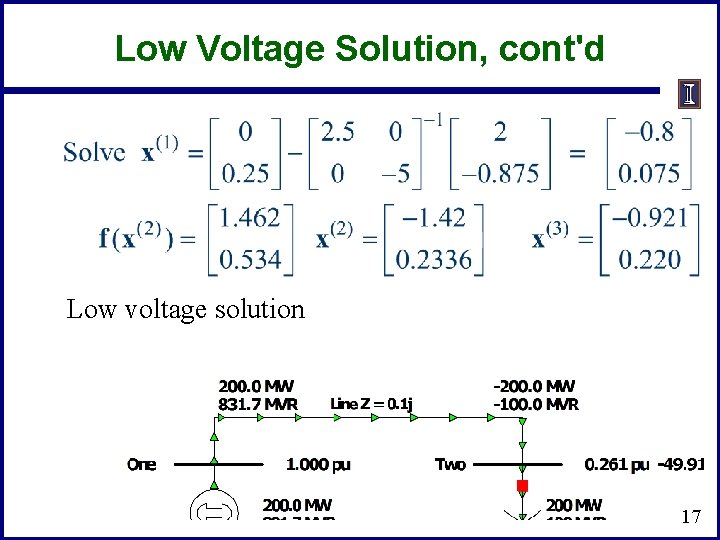
Low Voltage Solution, cont'd Low voltage solution 17

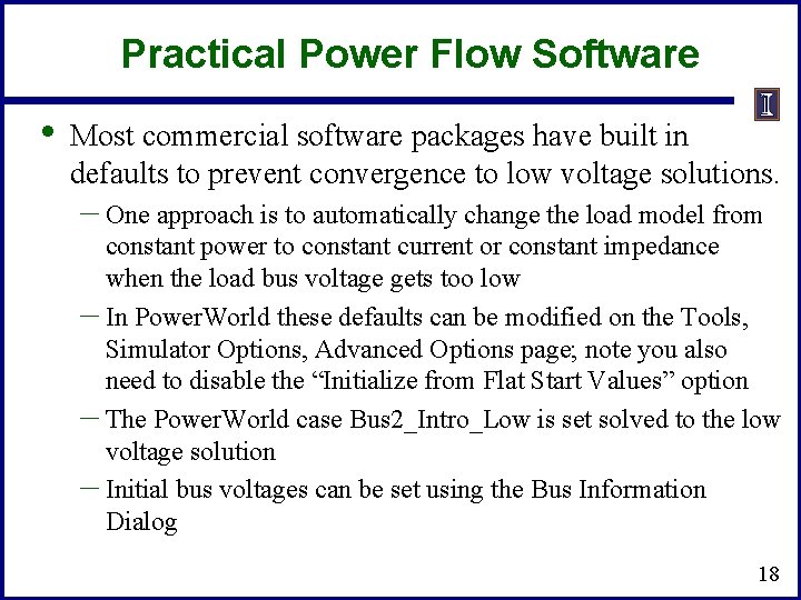
Practical Power Flow Software • Most commercial software packages have built in defaults to prevent convergence to low voltage solutions. – One approach is to automatically change the load model from constant power to constant current or constant impedance when the load bus voltage gets too low – In Power. World these defaults can be modified on the Tools, Simulator Options, Advanced Options page; note you also need to disable the “Initialize from Flat Start Values” option – The Power. World case Bus 2_Intro_Low is set solved to the low voltage solution – Initial bus voltages can be set using the Bus Information Dialog 18

NR Initialization • • • A textbook starting solution for the NR is to use “flat start” values in which all the angles are set to the slack bus angle, all the PQ bus voltages are set to 1. 0, and all the PV bus voltages are set to their PV setpoint values This approach usually works for small systems It seldom works for large systems. The usual approach for solving large systems is to start with an existing solution, modify it, then hope it converges – If not make the modification smaller – More robust methods are possible, but convergence is certainly not guaranteed!! 19

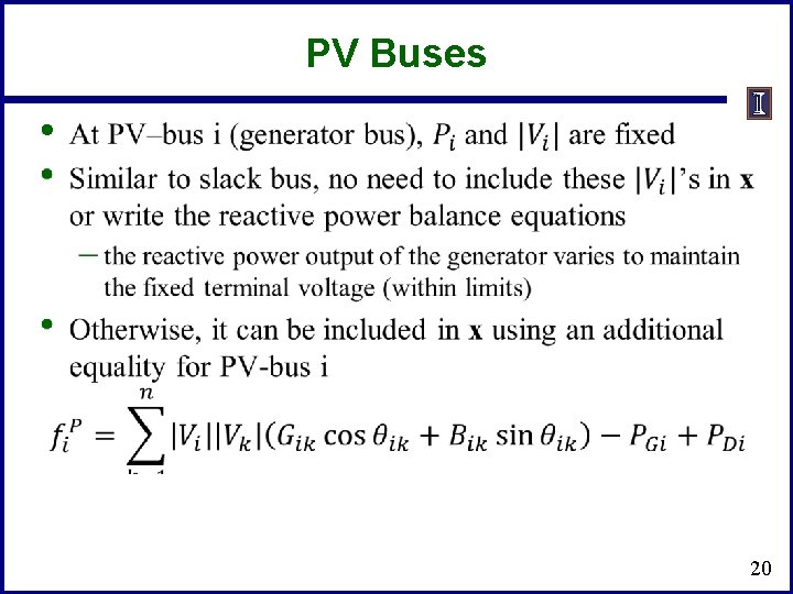
PV Buses • 20

Three Bus PV Case Example 21

Modeling Voltage Dependent Load 22

Voltage Dependent Load Example 23

Voltage Dependent Load, cont'd 24

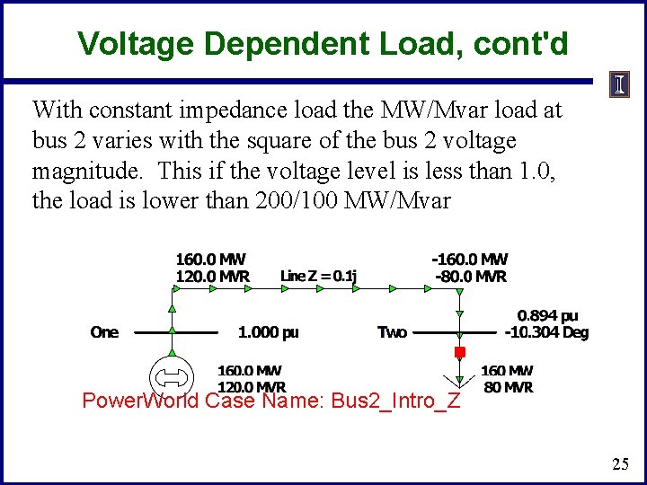
Voltage Dependent Load, cont'd With constant impedance load the MW/Mvar load at bus 2 varies with the square of the bus 2 voltage magnitude. This if the voltage level is less than 1. 0, the load is lower than 200/100 MW/Mvar Power. World Case Name: Bus 2_Intro_Z 25

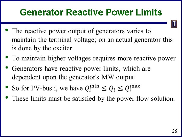
Generator Reactive Power Limits • 26

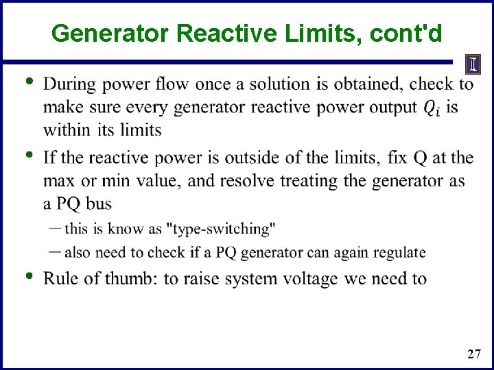
Generator Reactive Limits, cont'd • 27

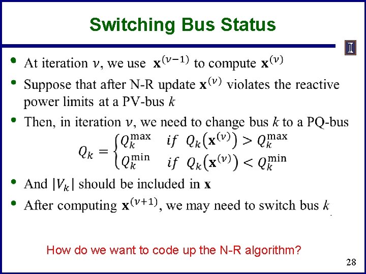
Switching Bus Status • How do we want to code up the N-R algorithm? 28

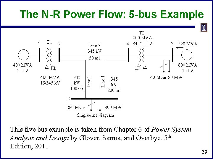
The N-R Power Flow: 5 -bus Example 1 T 1 5 T 2 800 MVA 4 345/15 k. V Line 3 345 k. V 50 mi 345 k. V 100 mi Line 1 400 MVA 15/345 k. V Line 2 400 MVA 15 k. V 345 k. V 200 mi 3 520 MVA 800 MVA 15 k. V 40 Mvar 80 MW 2 280 Mvar 800 MW Single-line diagram This five bus example is taken from Chapter 6 of Power System Analysis and Design by Glover, Sarma, and Overbye, 5 th Edition, 2011 29

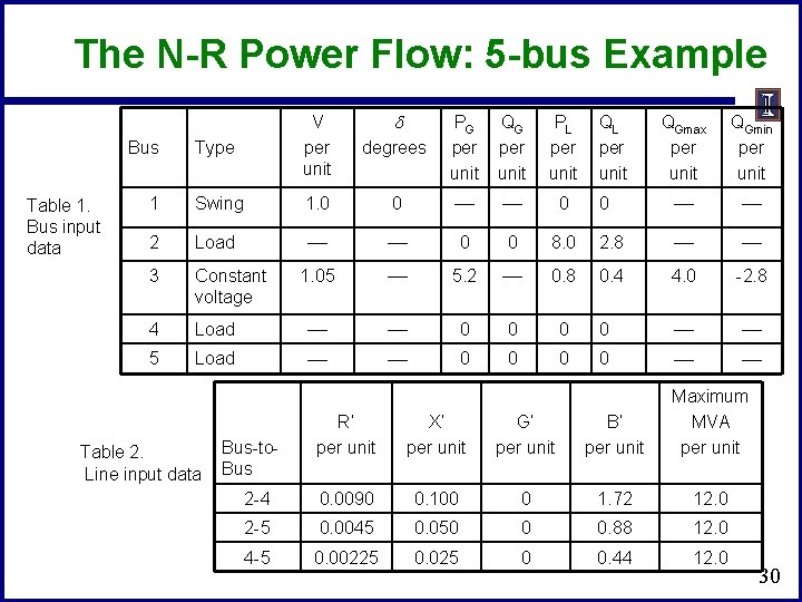
The N-R Power Flow: 5 -bus Example Type V per unit 1 Swing 2 Load 3 Constant voltage 4 5 Bus Table 1. Bus input data degrees PG per unit QG per unit PL per unit 1. 0 0 0 0 0 1. 05 5. 2 Load Table 2. Line input data QL per unit QGmax per unit QGmin per unit 0 8. 0 2. 8 0. 8 0. 4 4. 0 -2. 8 0 0 0 0 R’ per unit X’ per unit G’ per unit B’ per unit Maximum MVA per unit 2 -4 0. 0090 0. 100 0 1. 72 12. 0 2 -5 0. 0045 0. 050 0 0. 88 12. 0 4 -5 0. 00225 0. 025 0 0. 44 12. 0 Bus-to. Bus 30

The N-R Power Flow: 5 -bus Example Table 3. Transformer input data R per unit X per unit Gc per unit Bm per unit Maximum MVA per unit Maximum TAP Setting per unit 1 -5 0. 00150 0. 02 0 0 6. 0 — 3 -4 0. 00075 0. 01 0 0 10. 0 — Bus-to. Bus Table 4. Input data and unknowns Input Data Unknowns 1 V 1 = 1. 0, 1 = 0 P 1, Q 1 2 P 2 = PG 2 -PL 2 = -8 Q 2 = QG 2 -QL 2 = -2. 8 V 2, 2 3 V 3 = 1. 05 P 3 = PG 3 -PL 3 = 4. 4 Q 3, 3 4 P 4 = 0, Q 4 = 0 V 4, 4 5 P 5 = 0, Q 5 = 0 V 5, 5 31

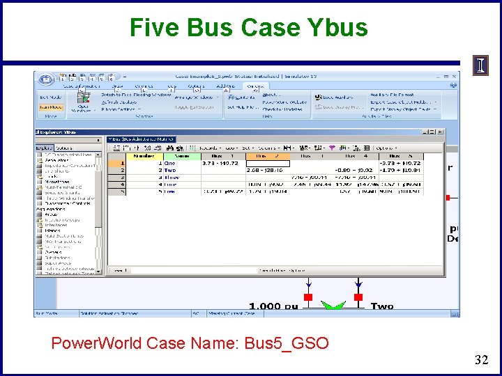
Five Bus Case Ybus Power. World Case Name: Bus 5_GSO 32

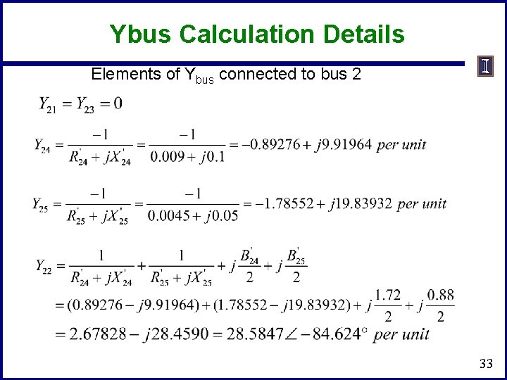
Ybus Calculation Details Elements of Ybus connected to bus 2 33

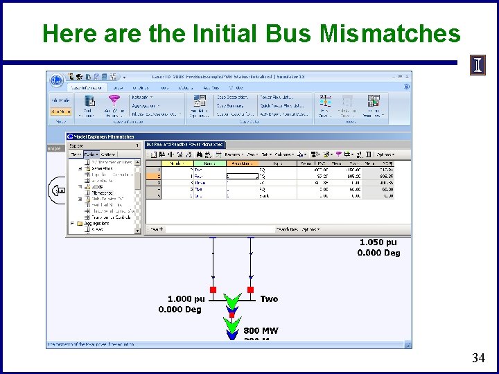
Here are the Initial Bus Mismatches 34

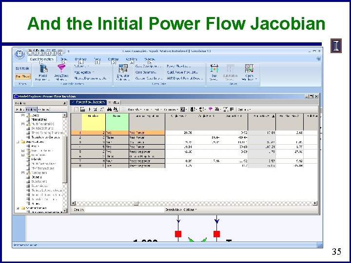
And the Initial Power Flow Jacobian 35

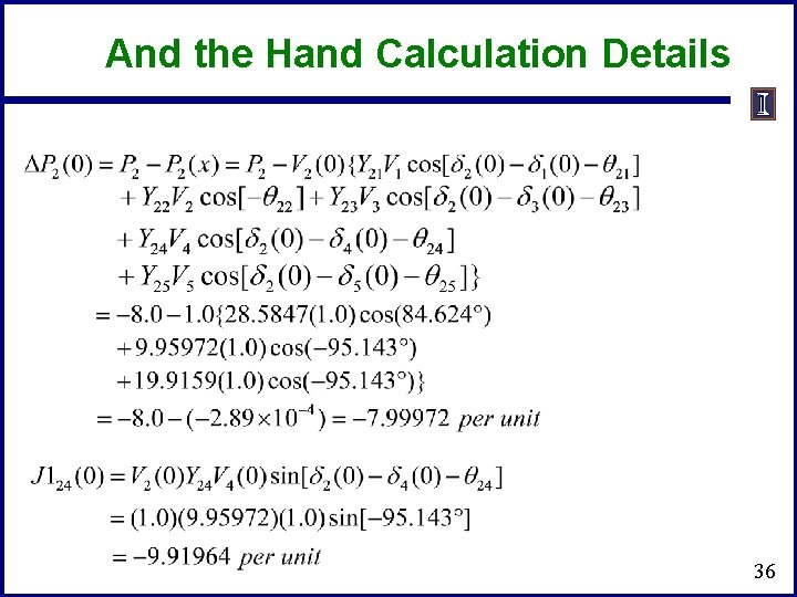
And the Hand Calculation Details 36

Five Bus Power System Solved 37

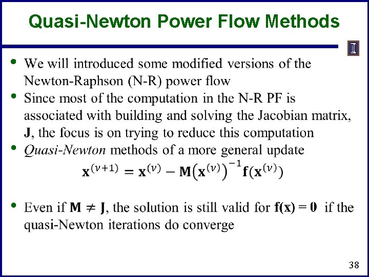
Quasi-Newton Power Flow Methods • 38

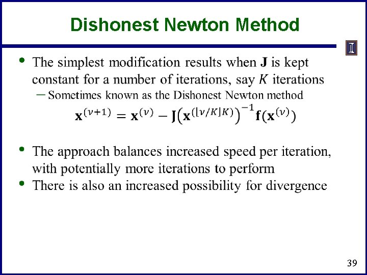
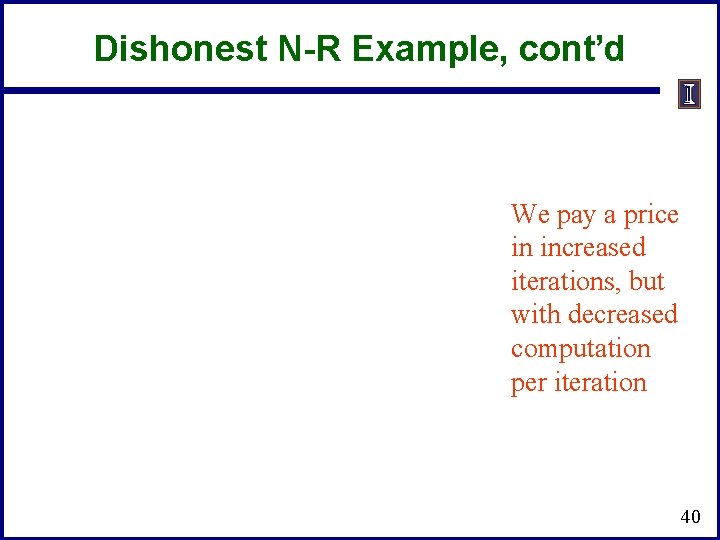
Dishonest Newton Method • 39

Dishonest N-R Example, cont’d We pay a price in increased iterations, but with decreased computation per iteration 40

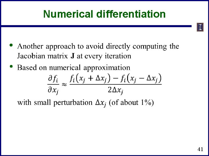
Numerical differentiation • 41

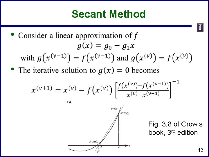
Secant Method • Fig. 3. 8 of Crow’s book, 3 rd edition 42