ECE 530 Analysis Techniques for LargeScale Electrical Systems

ECE 530 – Analysis Techniques for Large-Scale Electrical Systems Lecture 15: DC Power Flow Model; Sensitivity Analysis Prof. Hao Zhu Dept. of Electrical and Computer Engineering University of Illinois at Urbana-Champaign haozhu@illinois. edu 10/14/2014 1

Announcements • HW 5 is due October 21 • Midterm exam is October 23 in class; closed book and notes, but one 8. 5 by 11 inch note sheet and simple calculators allowed – Test covers up to dc power flow (before sensitivity) 2

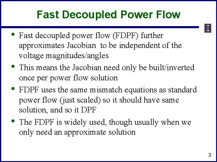
Fast Decoupled Power Flow • • Fast decoupled power flow (FDPF) further approximates Jacobian to be independent of the voltage magnitudes/angles This means the Jacobian need only be built/inverted once per power flow solution FDPF uses the same mismatch equations as standard power flow (just scaled) so it should have same solution, and so it DPF The FDPF is widely used, though usually when we only need an approximate solution 3

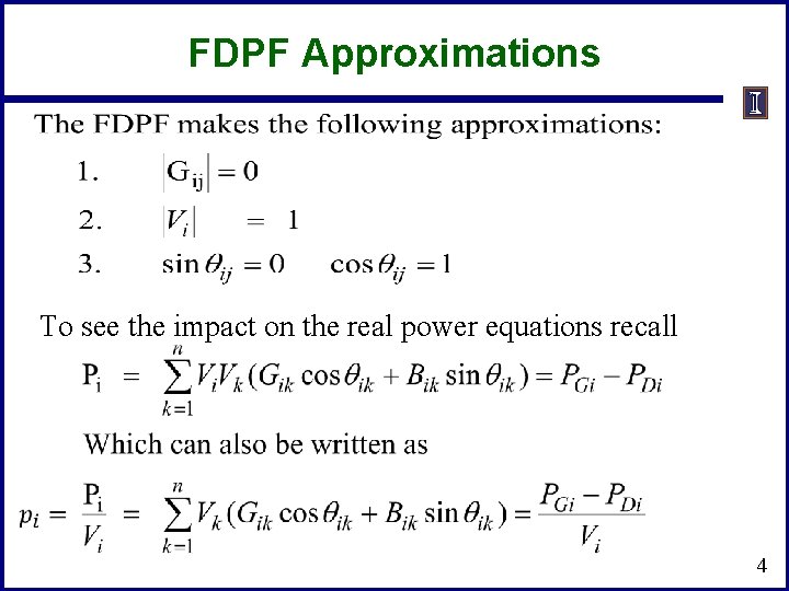
FDPF Approximations To see the impact on the real power equations recall 4

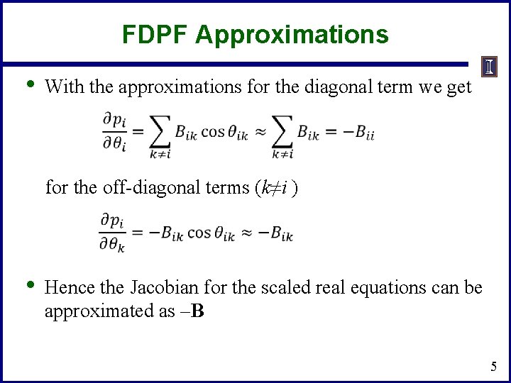
FDPF Approximations • With the approximations for the diagonal term we get for the off-diagonal terms (k≠i ) • Hence the Jacobian for the scaled real equations can be approximated as –B 5

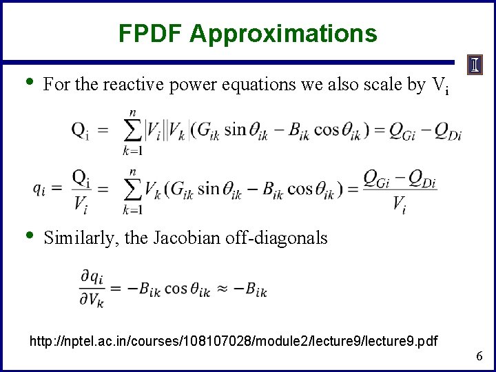
FPDF Approximations • For the reactive power equations we also scale by Vi • Similarly, the Jacobian off-diagonals http: //nptel. ac. in/courses/108107028/module 2/lecture 9. pdf 6

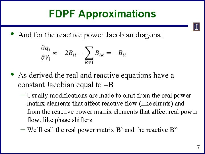
FDPF Approximations • And for the reactive power Jacobian diagonal • As derived the real and reactive equations have a constant Jacobian equal to –B – Usually modifications are made to omit from the real power matrix elements that affect reactive flow (like shunts) and from the reactive power matrix elements that affect real power flow, like phase shifters – We’ll call the real power matrix B’ and the reactive B” 7

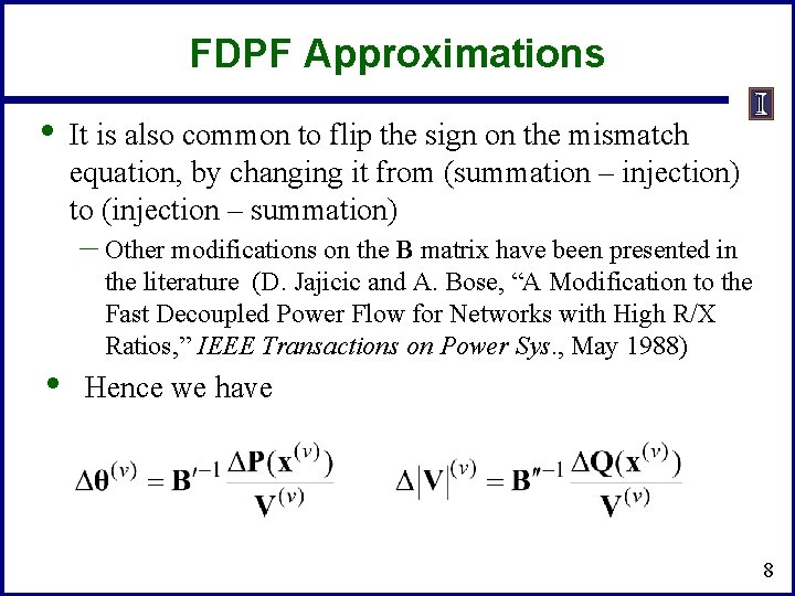
FDPF Approximations • It is also common to flip the sign on the mismatch equation, by changing it from (summation – injection) to (injection – summation) – Other modifications on the B matrix have been presented in • the literature (D. Jajicic and A. Bose, “A Modification to the Fast Decoupled Power Flow for Networks with High R/X Ratios, ” IEEE Transactions on Power Sys. , May 1988) Hence we have 8

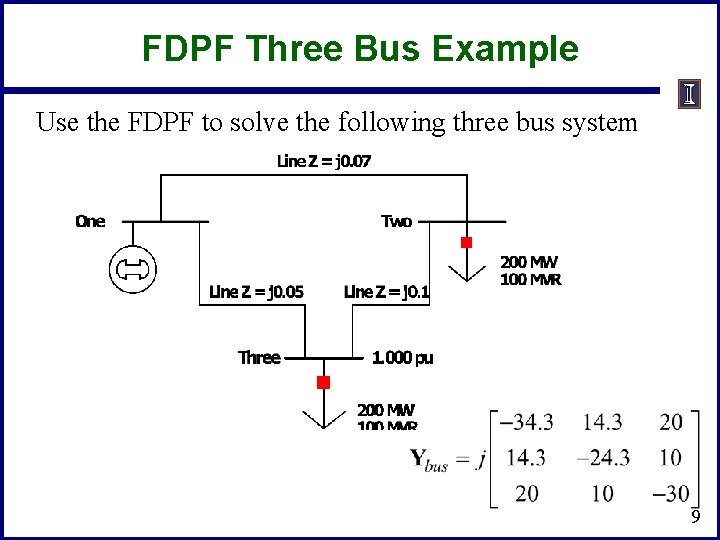
FDPF Three Bus Example Use the FDPF to solve the following three bus system 9

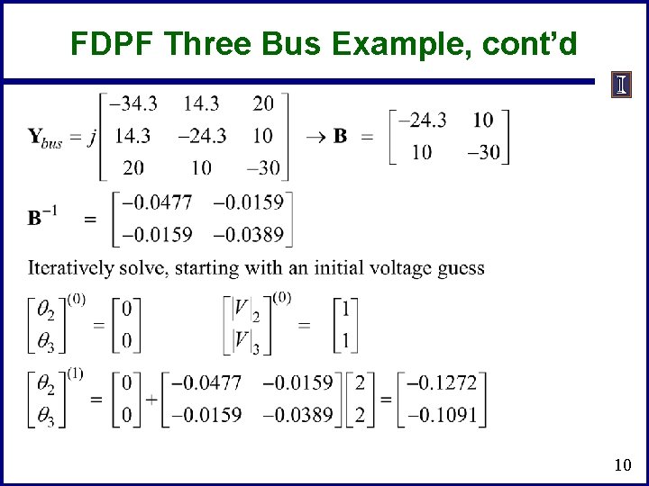
FDPF Three Bus Example, cont’d 10

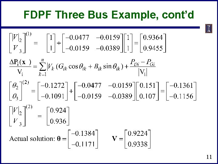
FDPF Three Bus Example, cont’d 11

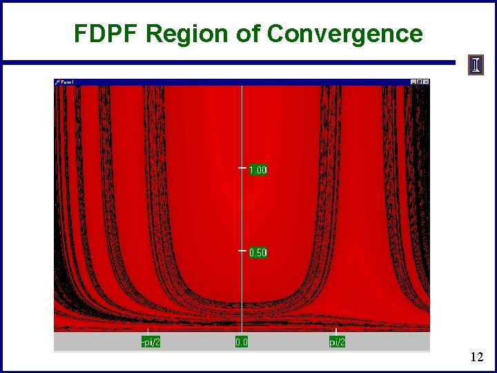
FDPF Region of Convergence 12

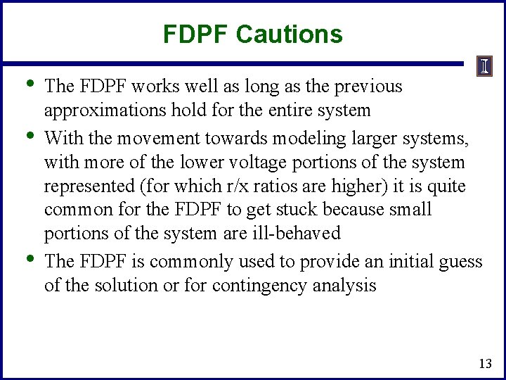
FDPF Cautions • • • The FDPF works well as long as the previous approximations hold for the entire system With the movement towards modeling larger systems, with more of the lower voltage portions of the system represented (for which r/x ratios are higher) it is quite common for the FDPF to get stuck because small portions of the system are ill-behaved The FDPF is commonly used to provide an initial guess of the solution or for contingency analysis 13

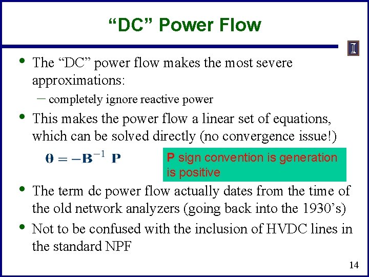
“DC” Power Flow • • The “DC” power flow makes the most severe approximations: – completely ignore reactive power This makes the power flow a linear set of equations, which can be solved directly (no convergence issue!) P sign convention is generation is positive The term dc power flow actually dates from the time of the old network analyzers (going back into the 1930’s) Not to be confused with the inclusion of HVDC lines in the standard NPF 14

DC Power Flow References • • • A nice formulation is given in the Power Generation and Control book by Wood and Wollenberg (with the 3 rd edition out) The August 2009 paper in IEEE Transactions on Power Systems, “DC Power Flow Revisited” (by Stott, Jardim and Alsac) provides good coverage T. J. Overbye, X. Cheng, and Y. Sun, “A comparison of the AC and DC power flow models for LMP Calculations, ” in Proc. 37 th Hawaii Int. Conf. System Sciences, 2004, compares the accuracy of the approach 15

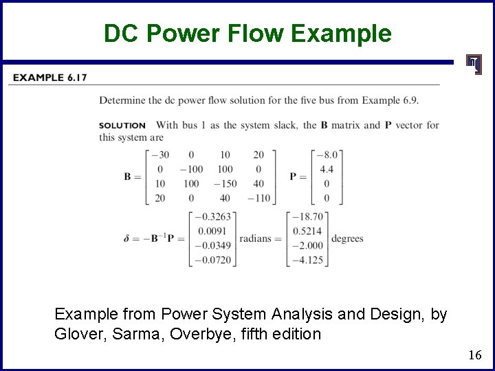
DC Power Flow Example from Power System Analysis and Design, by Glover, Sarma, Overbye, fifth edition 16

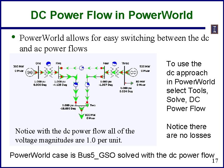
DC Power Flow in Power. World • Power. World allows for easy switching between the dc and ac power flows To use the dc approach in Power. World select Tools, Solve, DC Power Flow Notice with the dc power flow all of the voltage magnitudes are 1. 0 per unit. Notice there are no losses Power. World case is Bus 5_GSO solved with the dc power flow 17

Sensitivity Analysis • • • System description and notations Motivation for the sensitivity analysis From sensitivity to distribution factors Definitions of the various distribution factors Analysis of the distribution factors Distribution factor applications 18

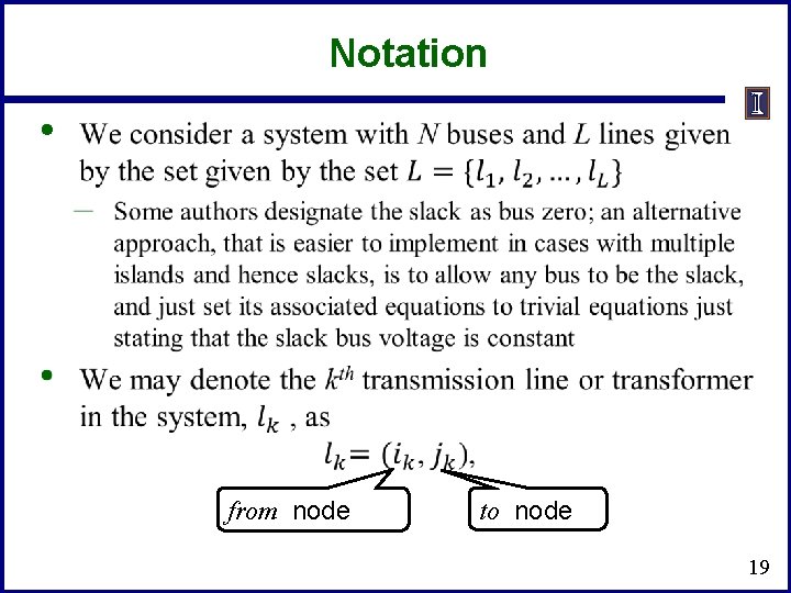
Notation • from node to node 19

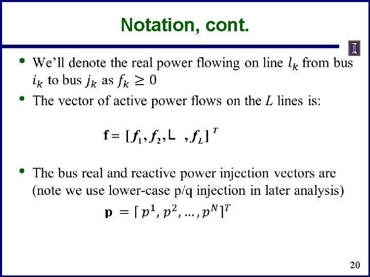
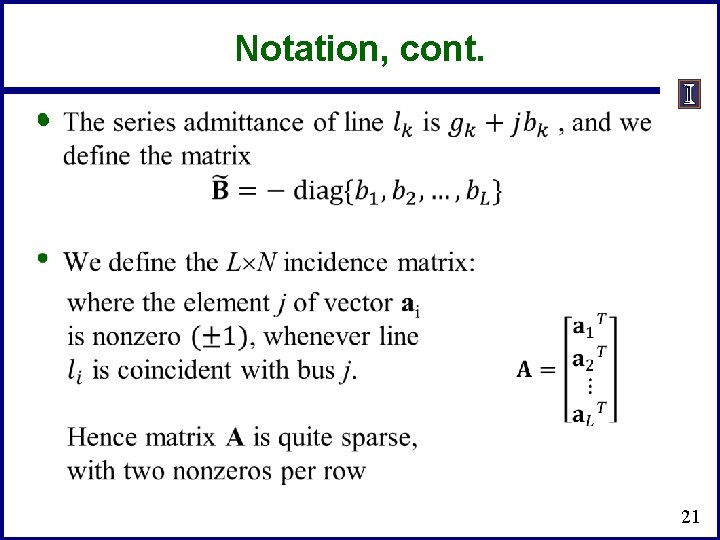
Notation, cont. • 20

Notation, cont. • 21

Analysis Example: Available Transfer Capability • • • The power system available transfer capability (ATC) is defined as the maximum additional MW that can be transferred between two specific areas, while meeting all the specified pre- and post-contingency system conditions ATC impacts measurably the market outcomes and system reliability and, therefore, the ATC values impact the system and market behavior A useful reference on ATC is Available Transfer Capability Definitions and Determination from NERC, June 1996 (available freely online) 22

ATC and Its Key Components • • • Total transfer capability (TTC ) – Amount of real power that can be transmitted across an interconnected transmission network in a reliable manner, including considering contingencies Transmission reliability margin (TRM) – Amount of TTC needed to deal with uncertainties in system conditions; typically expressed as a percent of TTC Capacity benefit margin (CBM) – Amount of TTC needed by load serving entities to ensure access to generation; typically expressed as a percent of TTC 23

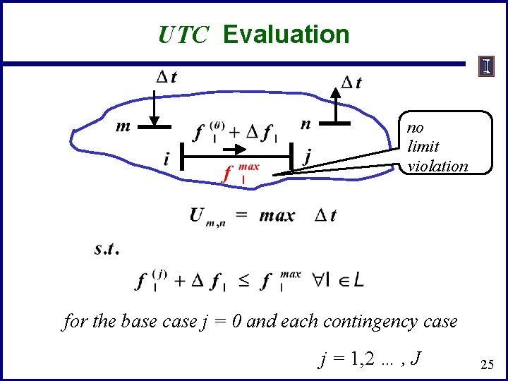
ATC and Its Key Components • • Uncommitted transfer capability (UTC) UTC = TTC – existing transmission commitments Formal definition of ATC is ATC = UTC – CBM – TRM We focus on determining Um, n, the UTC from node m to node n Um, n is defined as the maximum additional MW that can be transferred from node m to node n without violating any limit in either the base case or in any postcontingency conditions 24

UTC Evaluation no limit violation for the base case j = 0 and each contingency case j = 1, 2 … , J 25

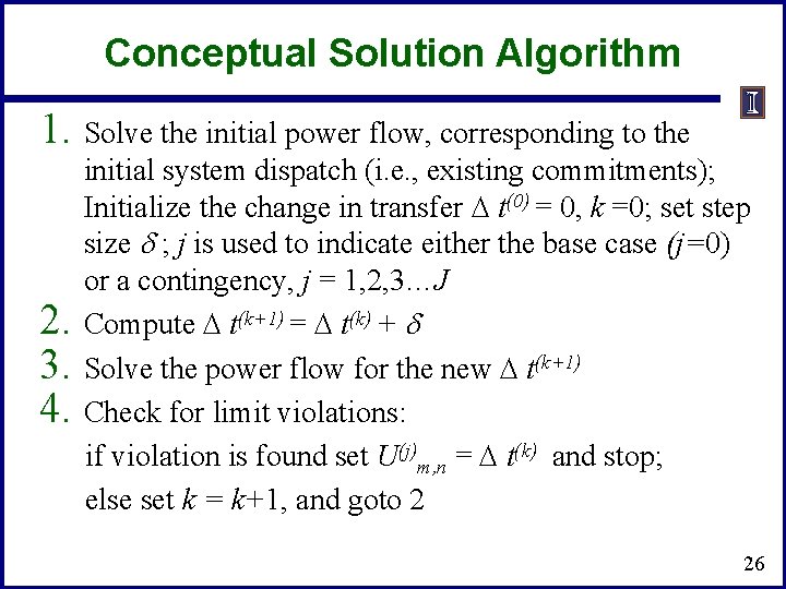
Conceptual Solution Algorithm 1. Solve the initial power flow, corresponding to the initial system dispatch (i. e. , existing commitments); Initialize the change in transfer t(0) = 0, k =0; set step size d ; j is used to indicate either the base case (j=0) or a contingency, j = 1, 2, 3…J 2. Compute t(k+1) = t(k) + d 3. Solve the power flow for the new t(k+1) 4. Check for limit violations: if violation is found set U(j)m, n = t(k) and stop; else set k = k+1, and goto 2 26

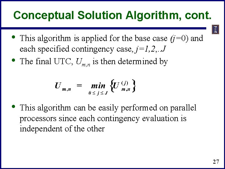
Conceptual Solution Algorithm, cont. • • • This algorithm is applied for the base case (j=0) and each specified contingency case, j=1, 2, . . J The final UTC, Um, n is then determined by This algorithm can be easily performed on parallel processors since each contingency evaluation is independent of the other 27

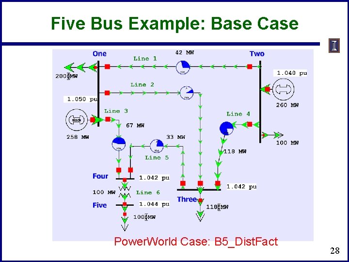
Five Bus Example: Base Case Power. World Case: B 5_Dist. Fact 28

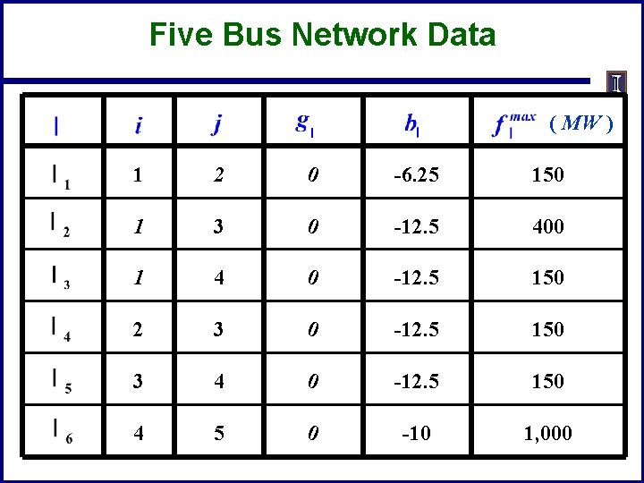
Five Bus Network Data ( MW ) 1 2 0 -6. 25 150 1 3 0 -12. 5 400 1 4 0 -12. 5 150 2 3 0 -12. 5 150 3 4 0 -12. 5 150 4 5 0 -10 1, 000

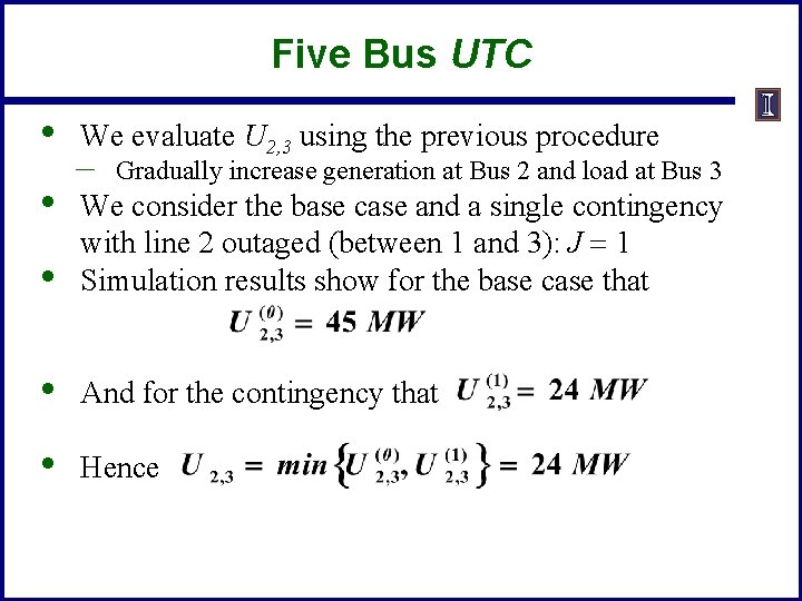
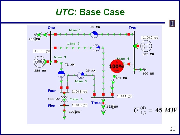
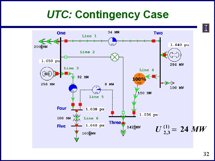
Five Bus UTC • • We evaluate U 2, 3 using the previous procedure – Gradually increase generation at Bus 2 and load at Bus 3 • We consider the base case and a single contingency with line 2 outaged (between 1 and 3): J = 1 Simulation results show for the base case that • And for the contingency that • Hence

UTC: Base Case 31

UTC: Contingency Case 32

Computational Considerations • • Obviously such a brute force approach can run into computational issues with large systems Consider the following situation: – – – 10 iterations for each case 6, 000 contingencies 2 seconds to solve each power flow It will take over 33 hours to compute a single UTC for the specified transfer direction from m to n. Consequently, there is an urgent need to develop fast tools that can provide satisfactory approximations 33