ECE 53 A Introduction to Analog and Digital

ECE 53 A Introduction to Analog and Digital Circuits Lecture Notes Second-Order Analog Circuit and System

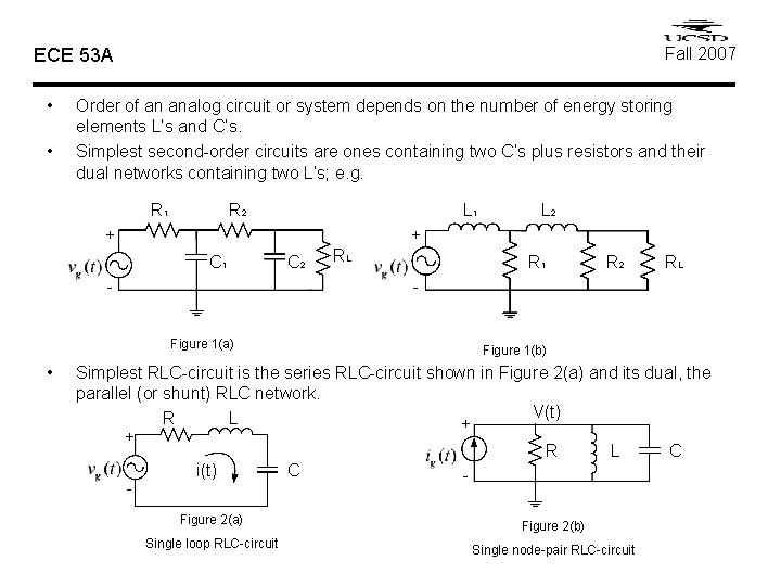
Fall 2007 ECE 53 A • • Order of an analog circuit or system depends on the number of energy storing elements L’s and C’s. Simplest second-order circuits are ones containing two C’s plus resistors and their dual networks containing two L’s; e. g. R 1 R 2 L 1 + + C 1 C 2 - RL R 1 R 2 RL - Figure 1(a) • L 2 Figure 1(b) Simplest RLC-circuit is the series RLC-circuit shown in Figure 2(a) and its dual, the parallel (or shunt) RLC network. V(t) R L + + R i(t) - C L - Figure 2(a) Figure 2(b) Single loop RLC-circuit Single node-pair RLC-circuit C

ECE 53 A Series-RLC Circuit R i. L(t) + Fall 2007 L + i(t) C Vc(t) - - Figure 1 Single-loop series RLC circuit First of all, even before we write the network equations to solve for the single unknown which is the loop current i(t), we need to satisfy two initial conditions (I. C) Vc(0) and i. L(0). KVL (loop) equation: [Note i. L(t)=i(t)] [Note ic(t)=i(t)] Differentiate Eq. (1) using (2), or

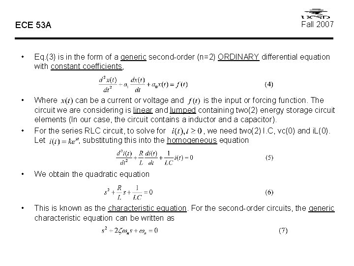
ECE 53 A Fall 2007 • Eq. (3) is in the form of a generic second-order (n=2) ORDINARY differential equation with constant coefficients, • Where can be a current or voltage and is the input or forcing function. The circuit we are considering is linear and lumped containing two(2) energy storage circuit elements (In our case, the circuit contains a inductor and a capacitor). For the series RLC circuit, to solve for , we need two(2) I. C, vc(0) and i. L(0). Let , substituting this into the homogeneous equation • • We obtain the quadratic equation • This is known as the characteristic equation. For the second-order circuits, the generic characteristic equation can be written as

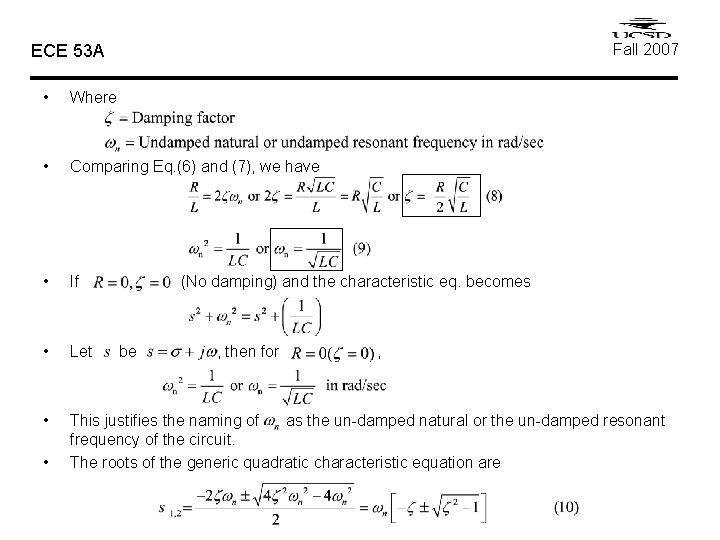
Fall 2007 ECE 53 A • Where • Comparing Eq. (6) and (7), we have • If • Let • This justifies the naming of as the un-damped natural or the un-damped resonant frequency of the circuit. The roots of the generic quadratic characteristic equation are • (No damping) and the characteristic eq. becomes be , then for ,

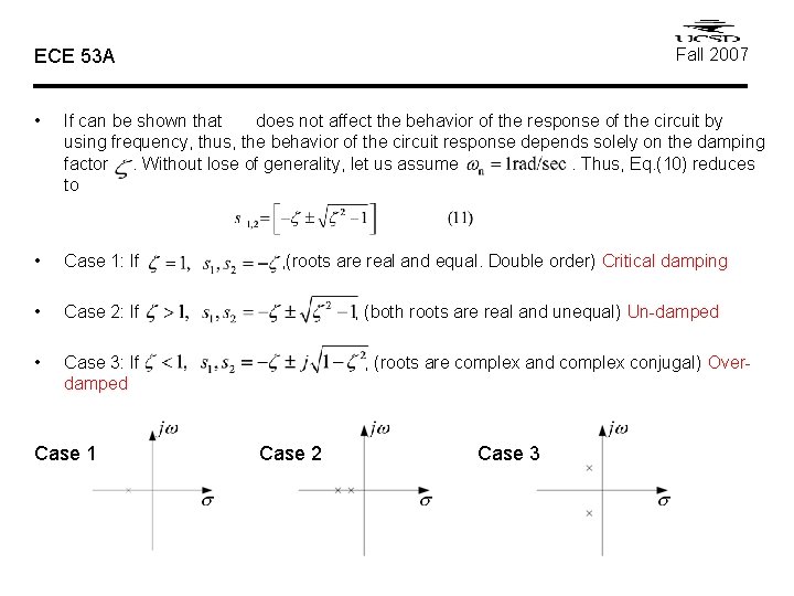
Fall 2007 ECE 53 A • If can be shown that does not affect the behavior of the response of the circuit by using frequency, thus, the behavior of the circuit response depends solely on the damping factor. Without lose of generality, let us assume. Thus, Eq. (10) reduces to • Case 1: If • Case 2: If • Case 3: If damped Case 1 , (roots are real and equal. Double order) Critical damping , (both roots are real and unequal) Un-damped , (roots are complex and complex conjugal) Over- Case 2 Case 3

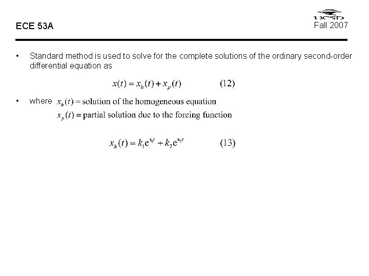
ECE 53 A Fall 2007 • Standard method is used to solve for the complete solutions of the ordinary second-order differential equation as • where

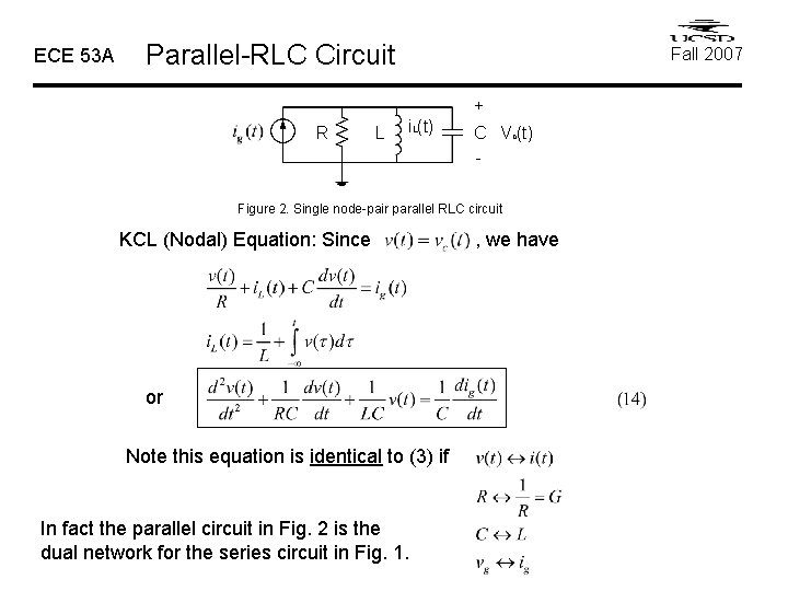
ECE 53 A Parallel-RLC Circuit Fall 2007 + R L i. L(t) C Vc(t) - Figure 2. Single node-pair parallel RLC circuit KCL (Nodal) Equation: Since or Note this equation is identical to (3) if In fact the parallel circuit in Fig. 2 is the dual network for the series circuit in Fig. 1. , we have

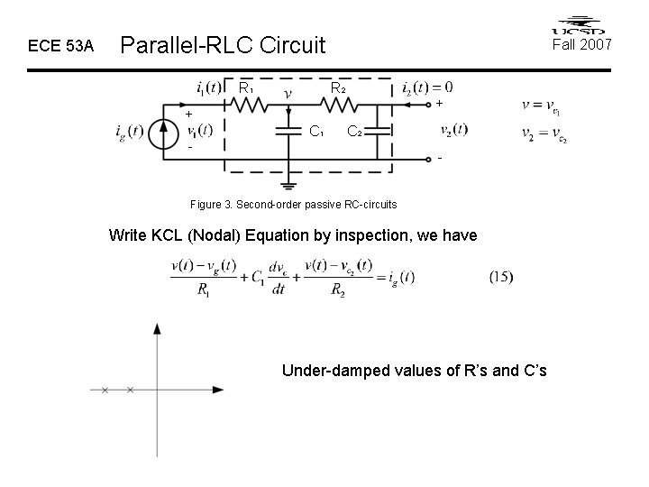
ECE 53 A Parallel-RLC Circuit R 1 Fall 2007 R 2 + + C 1 C 2 - - Figure 3. Second-order passive RC-circuits Write KCL (Nodal) Equation by inspection, we have Under-damped values of R’s and C’s

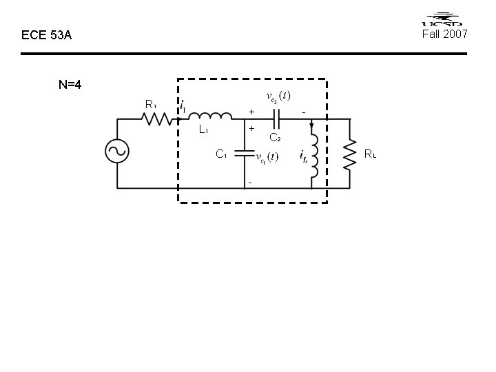
Fall 2007 ECE 53 A N=4 R 1 + + L 1 C 1 - C 2 RL -

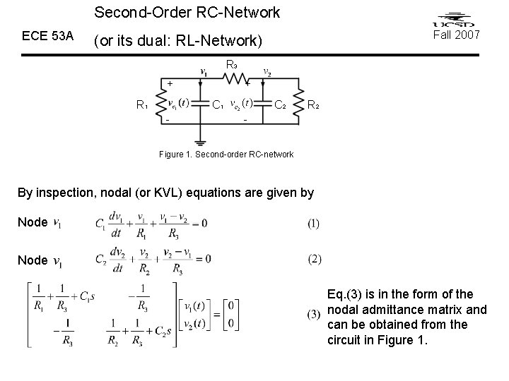
Second-Order RC-Network ECE 53 A Fall 2007 (or its dual: RL-Network) R 3 + R 1 + C 1 - C 2 R 2 - Figure 1. Second-order RC-network By inspection, nodal (or KVL) equations are given by Node Eq. (3) is in the form of the nodal admittance matrix and can be obtained from the circuit in Figure 1.

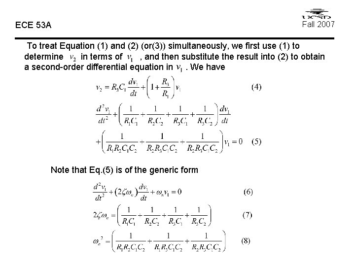
ECE 53 A Fall 2007 To treat Equation (1) and (2) (or(3)) simultaneously, we first use (1) to determine in terms of , and then substitute the result into (2) to obtain a second-order differential equation in. We have Note that Eq. (5) is of the generic form

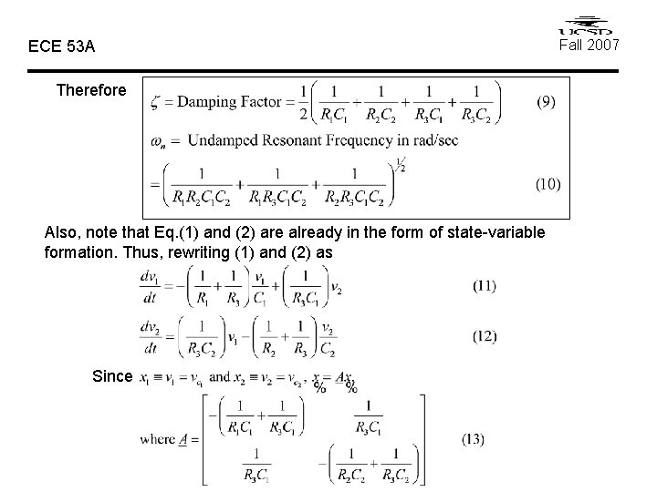
ECE 53 A Therefore Also, note that Eq. (1) and (2) are already in the form of state-variable formation. Thus, rewriting (1) and (2) as Since Fall 2007

ECE 53 A Fall 2007 For the special case of RC-network, the nodal equations are indeed the state equations using state variables. The roots of the characteristic equation are constrained to be only the negative -axis as shown below Where

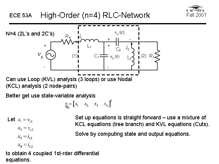
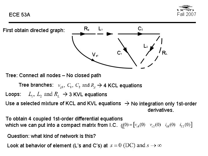
ECE 53 A High-Order (n=4) RLC-Network N=4 (2 L’s and 2 C’s) Rg + + + L 1 (1) C 1 - Fall 2007 - C 2 L 2 (2) RL - Can use Loop (KVL) analysis (3 loops) or use Nodal (KCL) analysis (2 node-pairs) Better get use state-variable analysis Let Set up equations is straight forward – use a mixture of KCL equations (tree branch) and KVL equations (Cuts). Solve by computing state and output equations. to obtain 4 coupled 1 st-rder differential equations.

Fall 2007 ECE 53 A First obtain directed graph: Rg L 1 C 2 L 2 Vg 1 C 1 RL Tree: Connect all nodes – No closed path Tree branches: Loops: 4 KCL equations 3 KVL equations Use a selected mixture of KCL and KVL equations No integration only 1 st-order derivatives. To obtain 4 coupled 1 st-order differential equations which we can put into a compact matrix from I. C. Question: what kind of network is this? Look at behavior of element (L’s and C’s) at

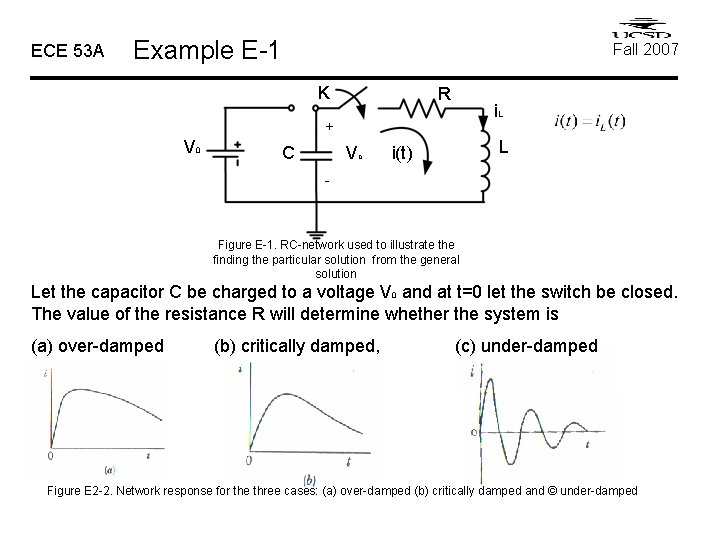
ECE 53 A Example E-1 Fall 2007 K R i. L + V 0 C Vc L i(t) - Figure E-1. RC-network used to illustrate the finding the particular solution from the general solution Let the capacitor C be charged to a voltage V 0 and at t=0 let the switch be closed. The value of the resistance R will determine whether the system is (a) over-damped (b) critically damped, (c) under-damped Figure E 2 -2. Network response for the three cases: (a) over-damped (b) critically damped and © under-damped

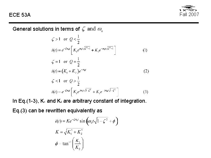
ECE 53 A General solutions in terms of In Eq. (1 -3), K 1 and K 2 are arbitrary constant of integration. Eq. (3) can be rewritten equivalently as Fall 2007

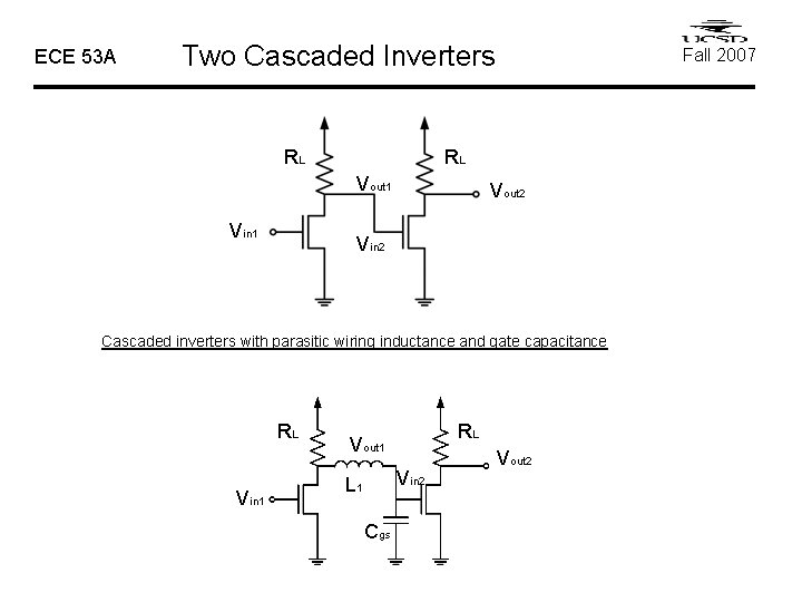
ECE 53 A Two Cascaded Inverters RL RL Vout 1 Vin 1 Fall 2007 Vout 2 Vin 2 Cascaded inverters with parasitic wiring inductance and gate capacitance RL Vin 1 RL Vout 1 Vin 2 L 1 Cgs Vout 2

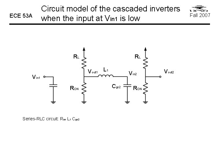
ECE 53 A Circuit model of the cascaded inverters when the input at Vin 1 is low RL RL Vout 1 Vin 1 RON Series-RLC circuit: Ron L 1 Cgs 2 L 1 Vin 2 Cgs 2 RON Vout 2 Fall 2007

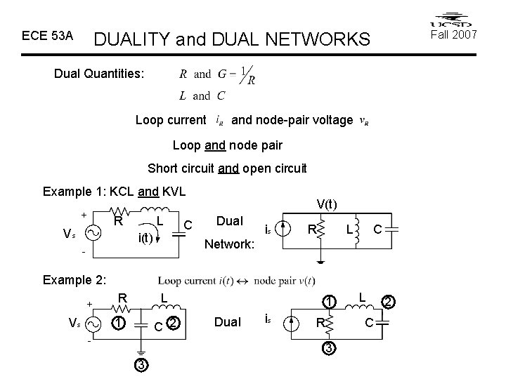
ECE 53 A Fall 2007 DUALITY and DUAL NETWORKS Dual Quantities: Loop current and node-pair voltage Loop and node pair Short circuit and open circuit Example 1: KCL and KVL + R Vs L i(t) C V(t) Dual is R L C Network: - Example 2: + Vs R L 1 C 2 - 1 Dual is R C 3 3 L 2

ECE 53 A State-variable method I. First-order circuits and systems For LTI systems, a, b, c, d are constants. II. Second-order circuits and systems For continuous-time LTI systems, A, B, C and D are constant matrices. For LTI analog lumped circuits containing R, L, C and transformers. I. C needed to solve the state equations: