ECE 476 POWER SYSTEM ANALYSIS Lecture 13 Power

ECE 476 POWER SYSTEM ANALYSIS Lecture 13 Power Flow Professor Tom Overbye Department of Electrical and Computer Engineering

Announcements l l Be reading Chapter 6, also Chapter 2. 4 (Network Equations). HW 5 is 2. 38, 6. 9, 6. 18, 6. 30, 6. 34, 6. 38; do by October 6 but does not need to be turned in. First exam is October 11 during class. Closed book, closed notes, one note sheet and calculators allowed. Exam covers thru the end of lecture 13 (today) An example previous exam (2008) is posted. Note this is exam was given earlier in the semester in 2008 so it did not include power flow, but the 2011 exam will (at least partially) 1

Multi-Variable Example 2

Multi-variable Example, cont’d 3

Multi-variable Example, cont’d 4

Possible EHV Overlays for Wind AEP 2007 Proposed Overlay 5

NR Application to Power Flow 6

Real Power Balance Equations 7

Newton-Raphson Power Flow 8

Power Flow Variables 9

N-R Power Flow Solution 10

Power Flow Jacobian Matrix 11

Power Flow Jacobian Matrix, cont’d 12

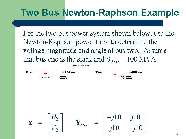
Two Bus Newton-Raphson Example For the two bus power system shown below, use the Newton-Raphson power flow to determine the voltage magnitude and angle at bus two. Assume that bus one is the slack and SBase = 100 MVA. 13

Two Bus Example, cont’d 14

Two Bus Example, cont’d 15

Two Bus Example, First Iteration 16

Two Bus Example, Next Iterations 17

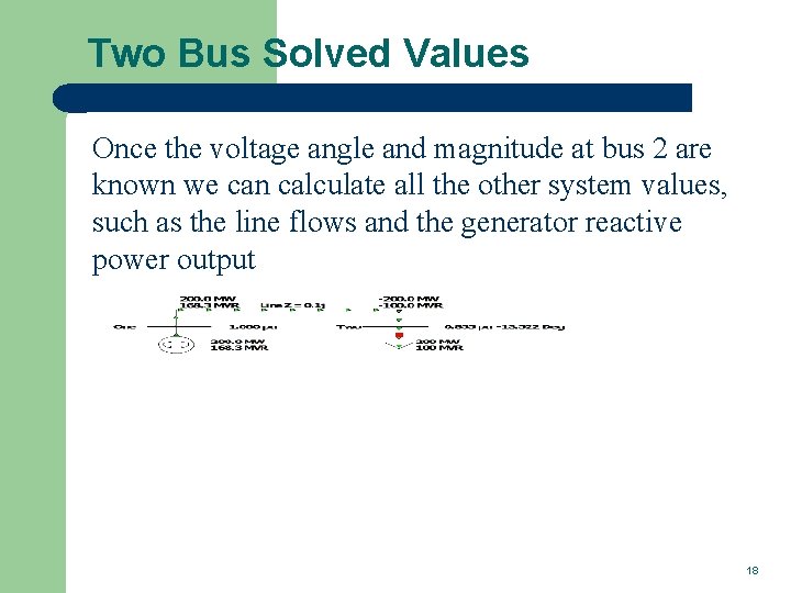
Two Bus Solved Values Once the voltage angle and magnitude at bus 2 are known we can calculate all the other system values, such as the line flows and the generator reactive power output 18

Two Bus Case Low Voltage Solution 19

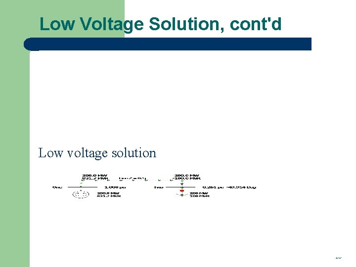
Low Voltage Solution, cont'd Low voltage solution 20

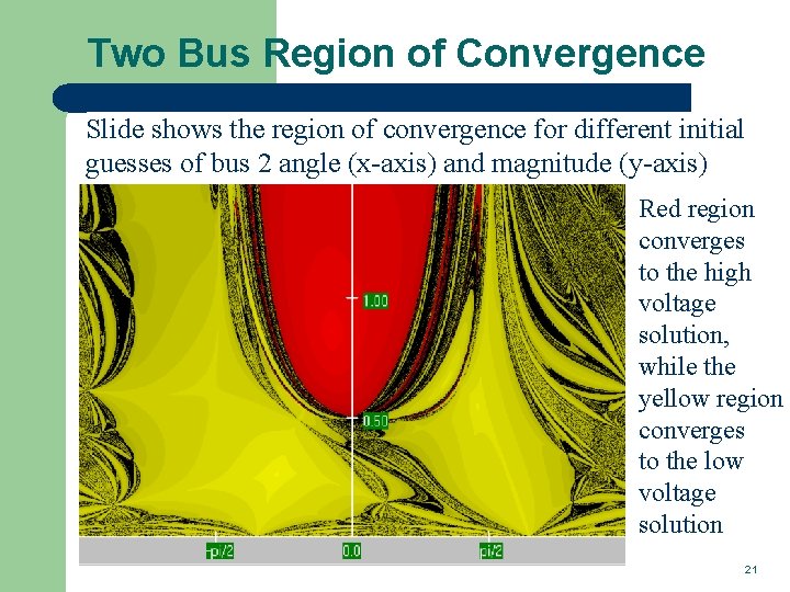
Two Bus Region of Convergence Slide shows the region of convergence for different initial guesses of bus 2 angle (x-axis) and magnitude (y-axis) Red region converges to the high voltage solution, while the yellow region converges to the low voltage solution 21

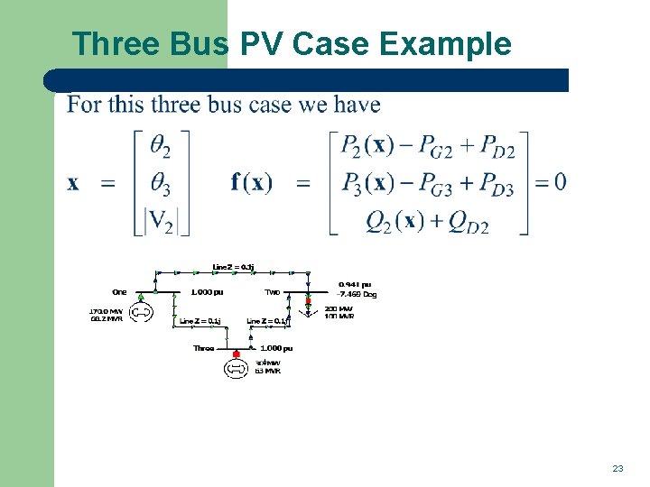
PV Buses l Since the voltage magnitude at PV buses is fixed there is no need to explicitly include these voltages in x or write the reactive power balance equations – – the reactive power output of the generator varies to maintain the fixed terminal voltage (within limits) optionally these variations/equations can be included by just writing the explicit voltage constraint for the generator bus |Vi | – Vi setpoint = 0 22

Three Bus PV Case Example 23

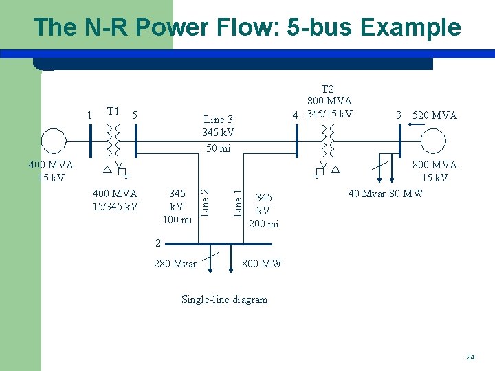
The N-R Power Flow: 5 -bus Example 1 T 1 5 T 2 800 MVA 4 345/15 k. V Line 3 345 k. V 50 mi 345 k. V 100 mi Line 1 400 MVA 15/345 k. V Line 2 400 MVA 15 k. V 345 k. V 200 mi 3 520 MVA 800 MVA 15 k. V 40 Mvar 80 MW 2 280 Mvar 800 MW Single-line diagram 24

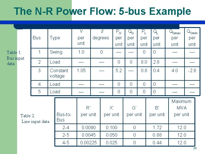
The N-R Power Flow: 5 -bus Example Type V per unit 1 Swing 2 Load 3 Constant voltage 4 5 Bus Table 1. Bus input data Table 2. Line input data degrees PG per unit QG per unit PL per unit 1. 0 0 0 0 0 1. 05 5. 2 Load QL per unit QGmax per unit QGmin per unit 0 8. 0 2. 8 0. 8 0. 4 4. 0 -2. 8 0 0 0 0 R’ per unit X’ per unit G’ per unit B’ per unit Maximum MVA per unit 2 -4 0. 0090 0. 100 0 1. 72 12. 0 2 -5 0. 0045 0. 050 0 0. 88 12. 0 4 -5 0. 00225 0. 025 0 0. 44 12. 0 Bus-to. Bus 25

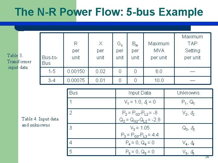
The N-R Power Flow: 5 -bus Example Table 3. Transformer input data R per unit X per unit Gc per unit Bm per unit Maximum MVA per unit Maximum TAP Setting per unit 1 -5 0. 00150 0. 02 0 0 6. 0 — 3 -4 0. 00075 0. 01 0 0 10. 0 — Bus-to. Bus Table 4. Input data and unknowns Input Data Unknowns 1 V 1 = 1. 0, 1 = 0 P 1, Q 1 2 P 2 = PG 2 -PL 2 = -8 Q 2 = QG 2 -QL 2 = -2. 8 V 2 , 2 3 V 3 = 1. 05 P 3 = PG 3 -PL 3 = 4. 4 Q 3 , 3 4 P 4 = 0, Q 4 = 0 V 4 , 4 5 P 5 = 0, Q 5 = 0 V 5 , 5 26

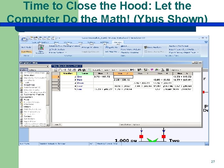
Time to Close the Hood: Let the Computer Do the Math! (Ybus Shown) 27

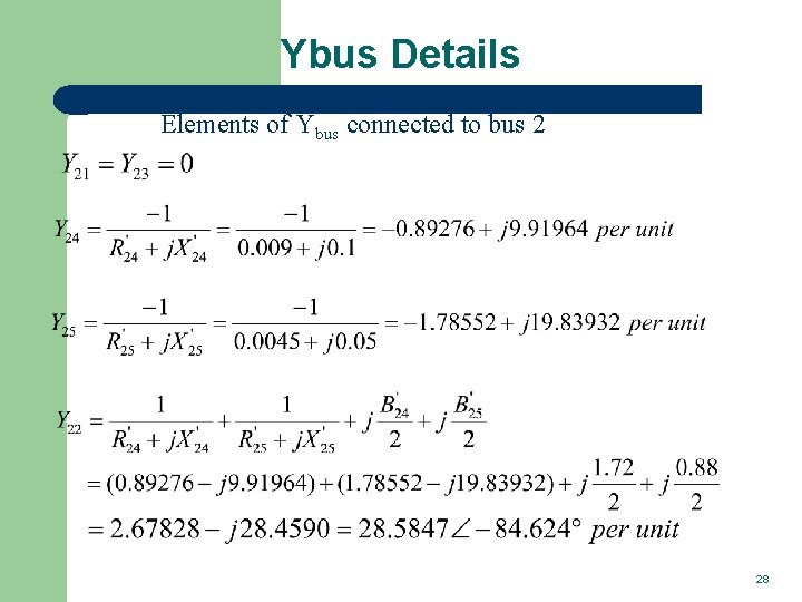
Ybus Details Elements of Ybus connected to bus 2 28

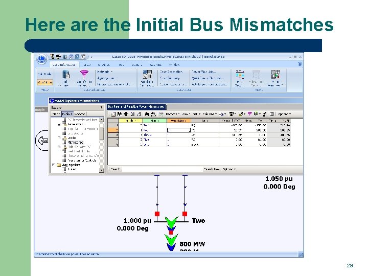
Here are the Initial Bus Mismatches 29

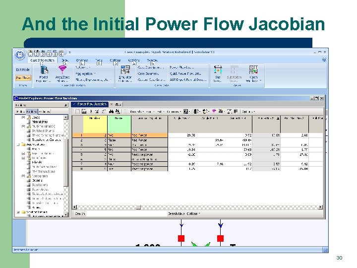
And the Initial Power Flow Jacobian 30

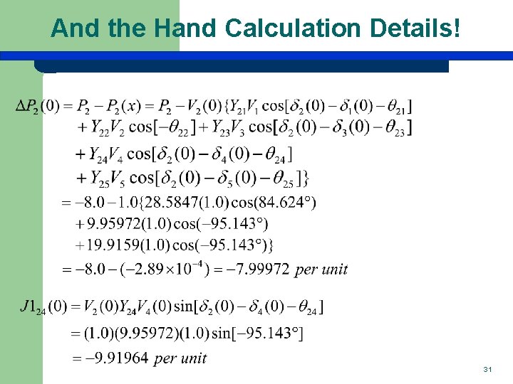
And the Hand Calculation Details! 31

Five Bus Power System Solved 32

37 Bus Example Design Case 33

Good Power System Operation • Good power system operation requires that there be no reliability violations for either the current condition or in the event of statistically likely contingencies • • • Reliability requires as a minimum that there be no transmission line/transformer limit violations and that bus voltages be within acceptable limits (perhaps 0. 95 to 1. 08) Example contingencies are the loss of any single device. This is known as n-1 reliability. North American Electric Reliability Corporation now has legal authority to enforce reliability standards (and there are now lots of them). See http: //www. nerc. com for details (click on Standards) 34

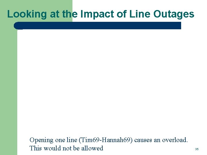
Looking at the Impact of Line Outages Opening one line (Tim 69 -Hannah 69) causes an overload. This would not be allowed 35

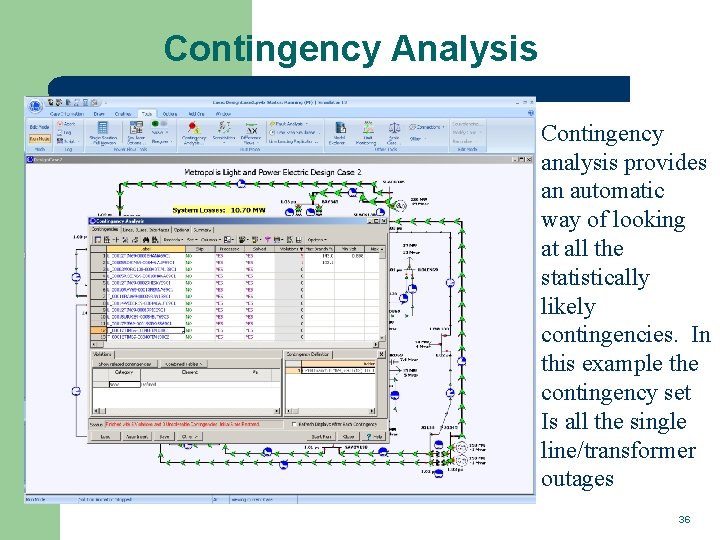
Contingency Analysis Contingency analysis provides an automatic way of looking at all the statistically likely contingencies. In this example the contingency set Is all the single line/transformer outages 36

Power Flow And Design • One common usage of the power flow is to determine how the system should be modified to remove contingencies problems or serve new load • • • In an operational context this requires working with the existing electric grid In a planning context additions to the grid can be considered In the next example we look at how to remove the existing contingency violations while serving new load. 37

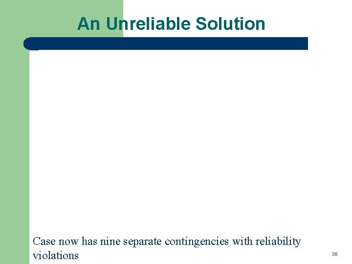
An Unreliable Solution Case now has nine separate contingencies with reliability violations 38

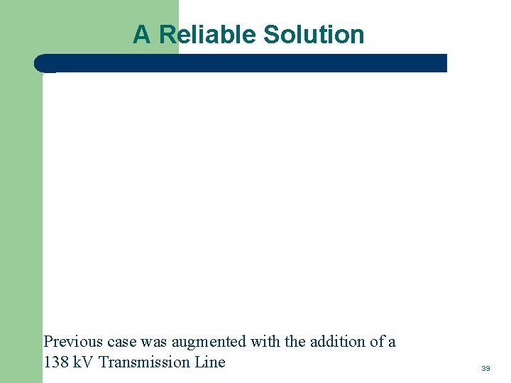
A Reliable Solution Previous case was augmented with the addition of a 138 k. V Transmission Line 39

Generation Changes and The Slack Bus • The power flow is a steady-state analysis tool, so the assumption is total load plus losses is always equal to total generation • • Generation mismatch is made up at the slack bus When doing generation change power flow studies one always needs to be cognizant of where the generation is being made up • Common options include system slack, distributed across multiple generators by participation factors or by economics 40

Generation Change Example 1 Display shows “Difference Flows” between original 37 bus case, and case with a BLT 138 generation outage; note all the power change is picked up at the slack 41

Generation Change Example 2 Display repeats previous case except now the change in generation is picked up by other generators using a participation factor approach 42

Voltage Regulation Example: 37 Buses Display shows voltage contour of the power system, demo will show the impact of generator voltage set point, reactive power limits, and switched capacitors 43

Solving Large Power Systems l The most difficult computational task is inverting the Jacobian matrix – – inverting a full matrix is an order n 3 operation, meaning the amount of computation increases with the cube of the size this amount of computation can be decreased substantially by recognizing that since the Ybus is a sparse matrix, the Jacobian is also a sparse matrix using sparse matrix methods results in a computational order of about n 1. 5. this is a substantial savings when solving systems with tens of thousands of buses 44

Newton-Raphson Power Flow l Advantages – – l Disadvantages – – l fast convergence as long as initial guess is close to solution large region of convergence each iteration takes much longer than a Gauss-Seidel iteration more complicated to code, particularly when implementing sparse matrix algorithms Newton-Raphson algorithm is very common in power flow analysis 45