ECE 476 Power System Analysis Lecture 12 Power



- Slides: 36

ECE 476 Power System Analysis Lecture 12: Power Flow Prof. Tom Overbye Dept. of Electrical and Computer Engineering University of Illinois at Urbana-Champaign overbye@illinois. edu

Announcements • Read Chapter 6 • H 6 is 6. 19, 6. 30, 6. 31, 6. 34, 6. 38, 6. 45. It does not need to be turned in, but will be covered by an in-class quiz on Oct 15. 1

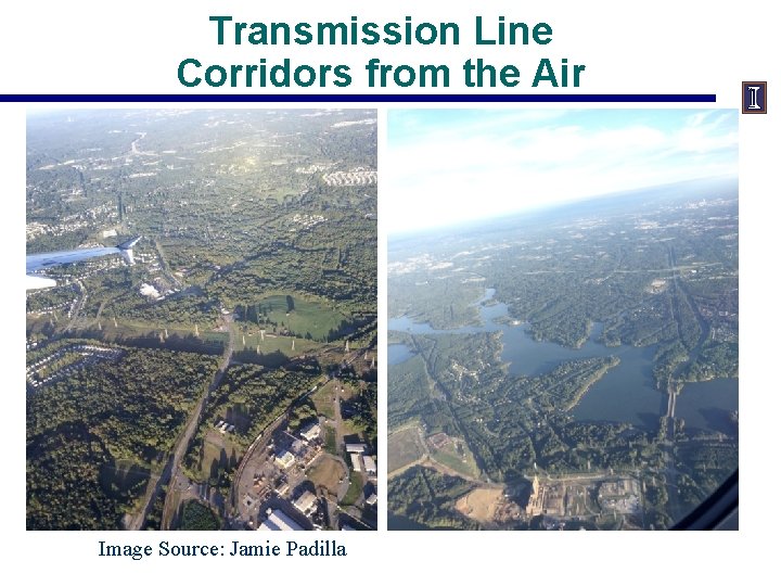
Transmission Line Corridors from the Air Image Source: Jamie Padilla

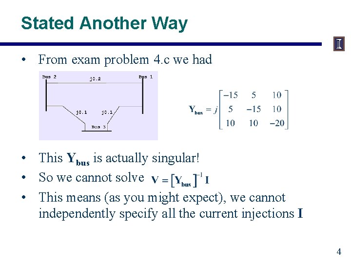
Slack Bus • In previous example we specified S 2 and V 1 and then solved for S 1 and V 2. • We can not arbitrarily specify S at all buses because total generation must equal total load + total losses • We also need an angle reference bus. • To solve these problems we define one bus as the "slack" bus. This bus has a fixed voltage magnitude and angle, and a varying real/reactive power injection. 3

Stated Another Way • From exam problem 4. c we had • This Ybus is actually singular! • So we cannot solve • This means (as you might expect), we cannot independently specify all the current injections I 4

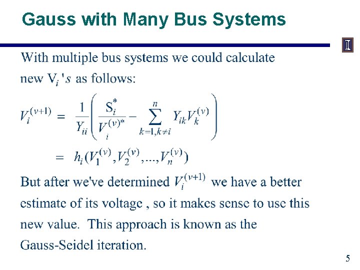
Gauss with Many Bus Systems 5

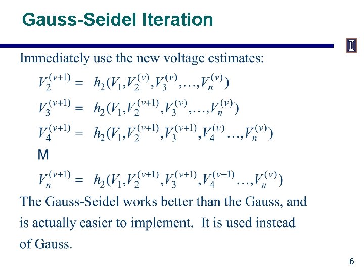
Gauss-Seidel Iteration 6

Three Types of Power Flow Buses • There are three main types of power flow buses – – – Load (PQ) at which P and Q are fixed; iteration solves for voltage magnitude and angle. Slack at which the voltage magnitude and angle are fixed; iteration solves for P and Q injections Generator (PV) at which P and |V| are fixed; iteration solves for voltage angle and Q injection • special coding is needed to include PV buses in the Gauss-Seidel iteration (covered in book, but not in slides since Gauss-Seidel is no longer commonly used) 7

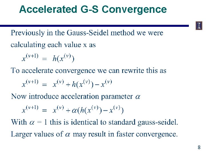
Accelerated G-S Convergence 8

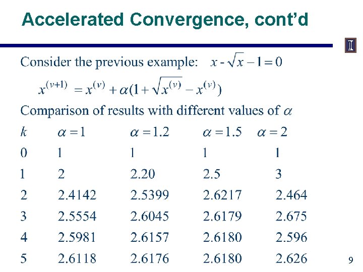
Accelerated Convergence, cont’d 9

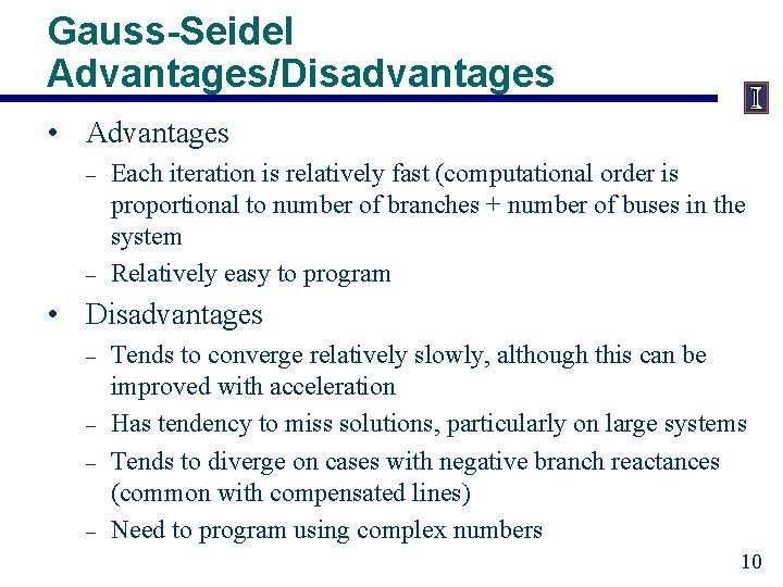
Gauss-Seidel Advantages/Disadvantages • Advantages – – Each iteration is relatively fast (computational order is proportional to number of branches + number of buses in the system Relatively easy to program • Disadvantages – – Tends to converge relatively slowly, although this can be improved with acceleration Has tendency to miss solutions, particularly on large systems Tends to diverge on cases with negative branch reactances (common with compensated lines) Need to program using complex numbers 10

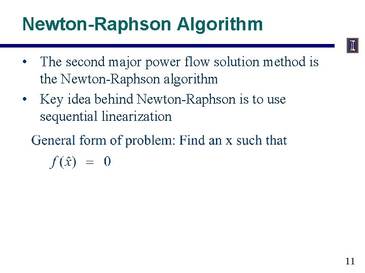
Newton-Raphson Algorithm • The second major power flow solution method is the Newton-Raphson algorithm • Key idea behind Newton-Raphson is to use sequential linearization 11

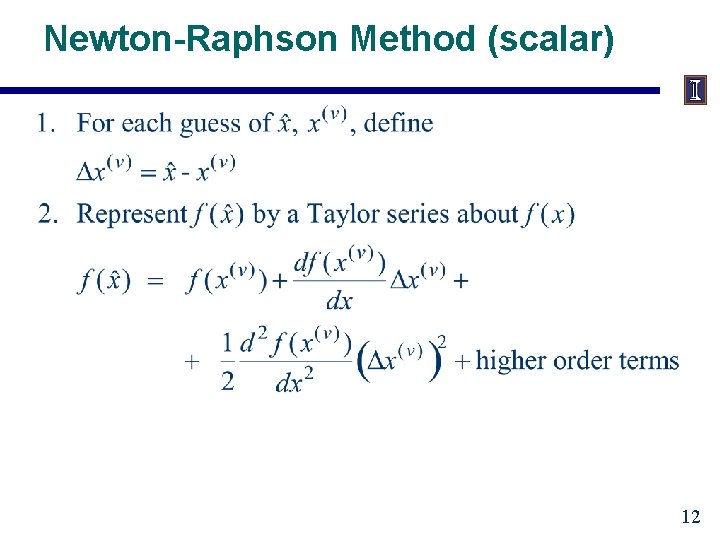
Newton-Raphson Method (scalar) 12

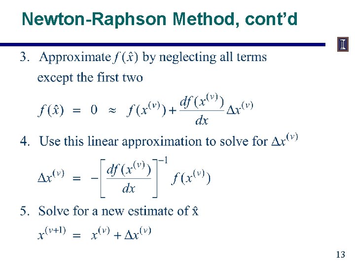
Newton-Raphson Method, cont’d 13

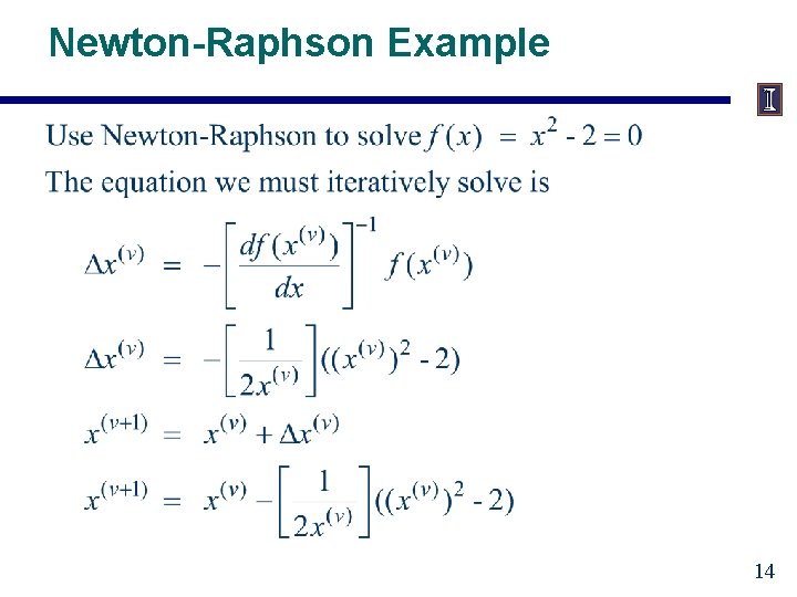
Newton-Raphson Example 14

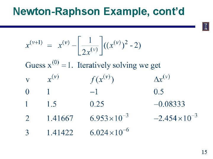
Newton-Raphson Example, cont’d 15

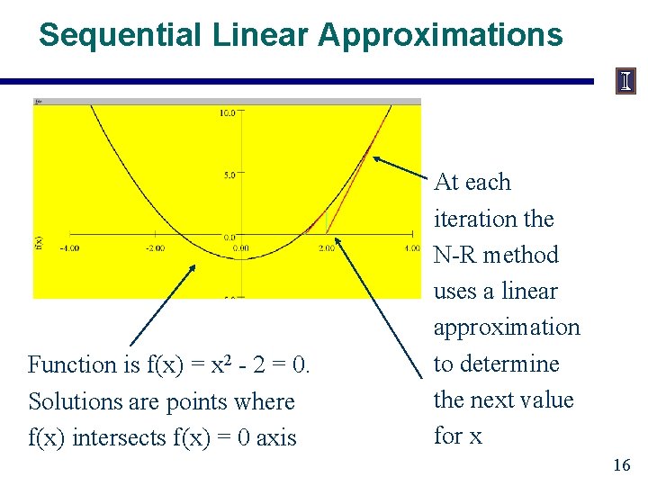
Sequential Linear Approximations Function is f(x) = x 2 - 2 = 0. Solutions are points where f(x) intersects f(x) = 0 axis At each iteration the N-R method uses a linear approximation to determine the next value for x 16

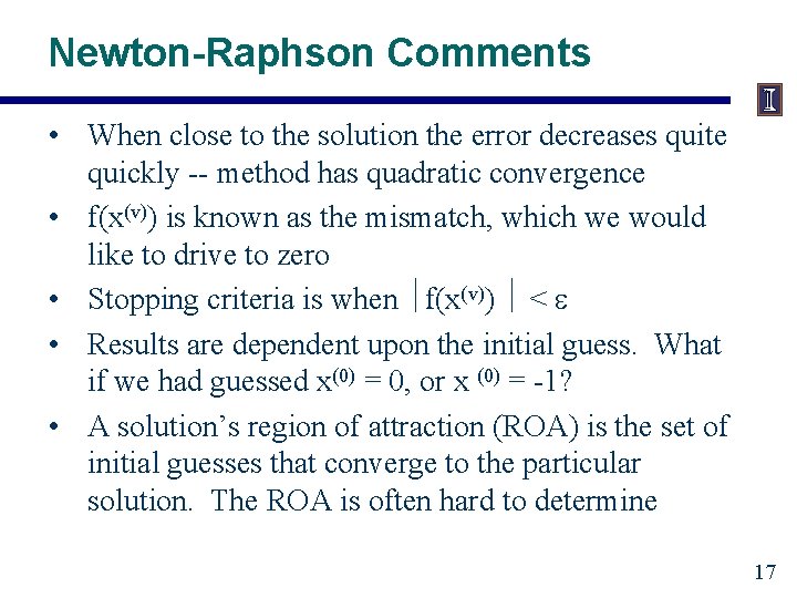
Newton-Raphson Comments • When close to the solution the error decreases quite quickly -- method has quadratic convergence • f(x(v)) is known as the mismatch, which we would like to drive to zero • Stopping criteria is when f(x(v)) < • Results are dependent upon the initial guess. What if we had guessed x(0) = 0, or x (0) = -1? • A solution’s region of attraction (ROA) is the set of initial guesses that converge to the particular solution. The ROA is often hard to determine 17

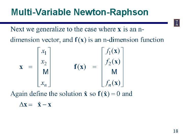
Multi-Variable Newton-Raphson 18

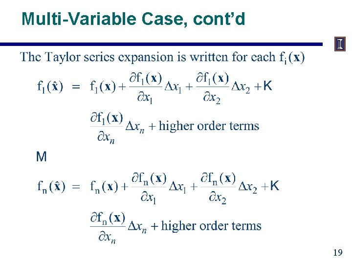
Multi-Variable Case, cont’d 19

Multi-Variable Case, cont’d 20

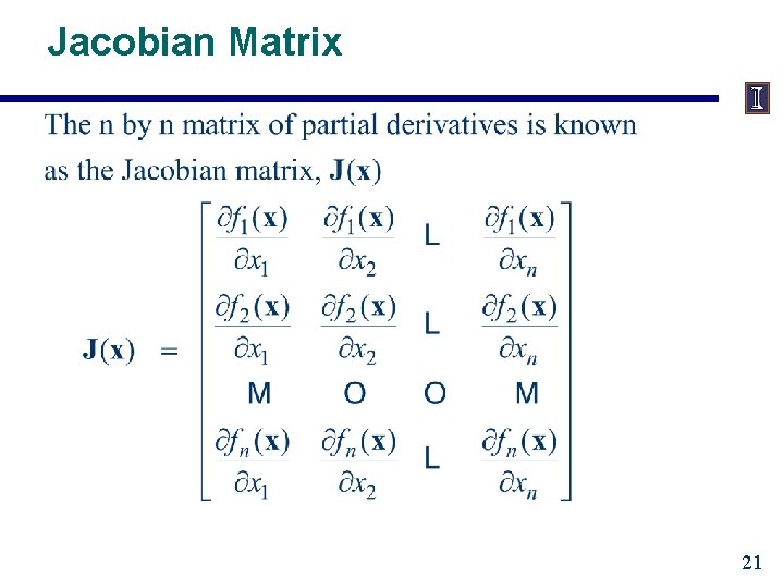
Jacobian Matrix 21

Multi-Variable Example 22

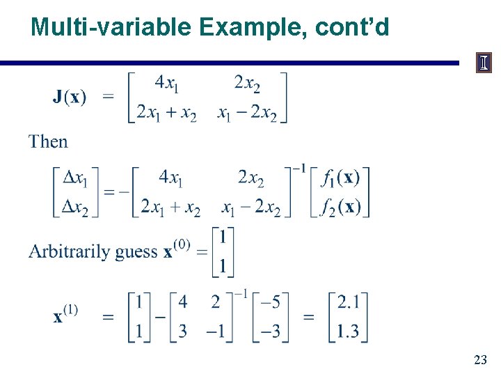
Multi-variable Example, cont’d 23

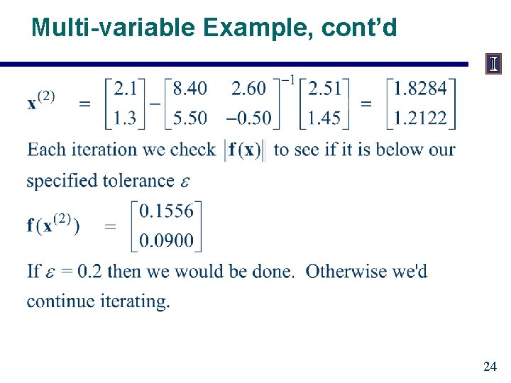
Multi-variable Example, cont’d 24

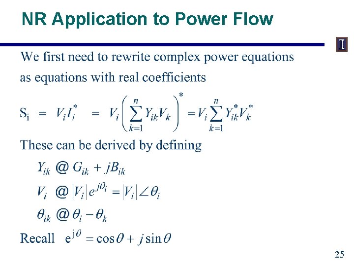
NR Application to Power Flow 25

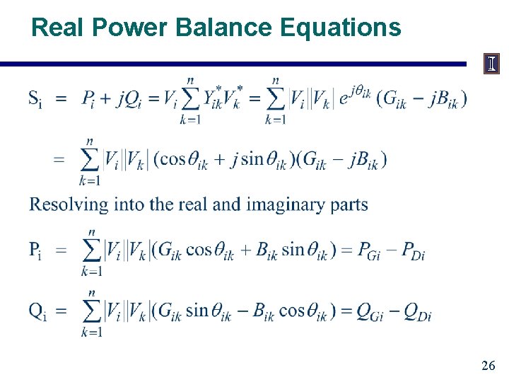
Real Power Balance Equations 26

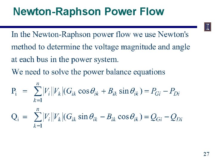
Newton-Raphson Power Flow 27

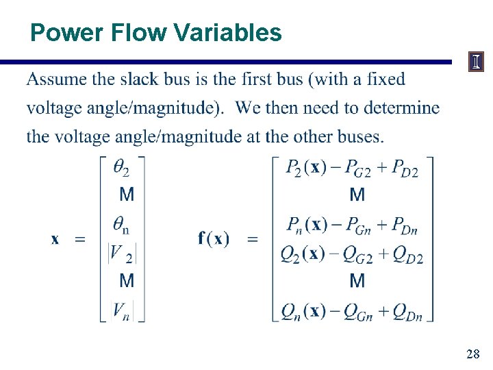
Power Flow Variables 28

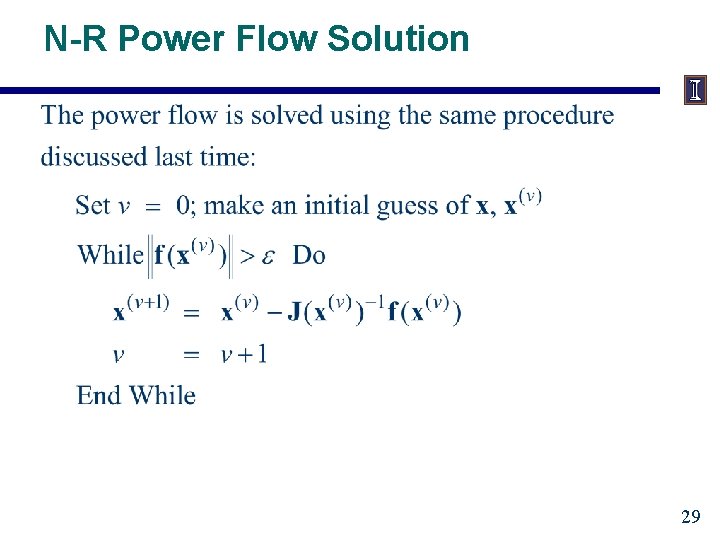
N-R Power Flow Solution 29

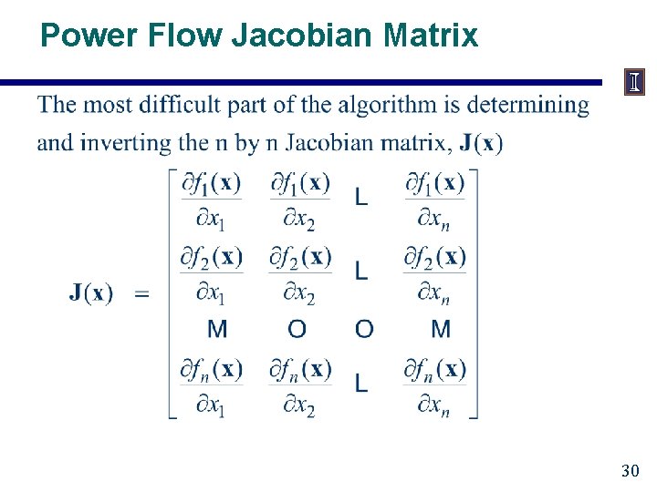
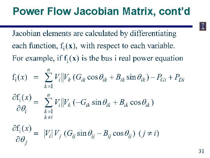
Power Flow Jacobian Matrix 30

Power Flow Jacobian Matrix, cont’d 31

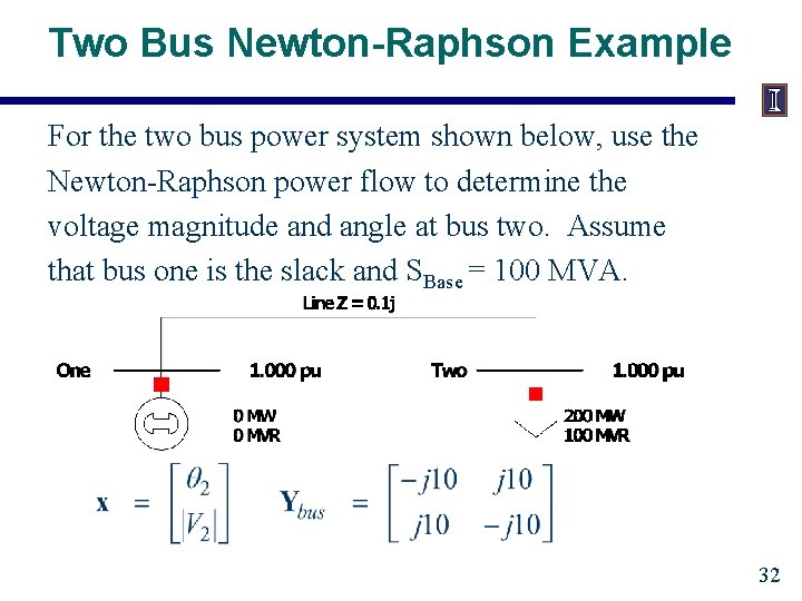
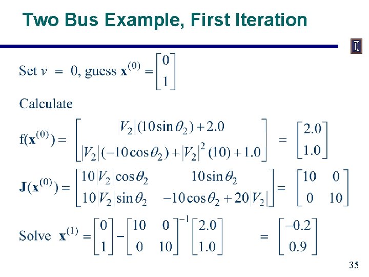
Two Bus Newton-Raphson Example For the two bus power system shown below, use the Newton-Raphson power flow to determine the voltage magnitude and angle at bus two. Assume that bus one is the slack and SBase = 100 MVA. 32

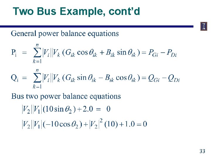
Two Bus Example, cont’d 33

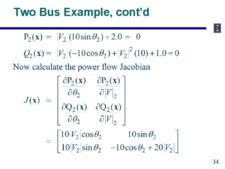
Two Bus Example, cont’d 34

Two Bus Example, First Iteration 35