ECE 368 Sequential Multiplication Shantanu Dutt ECE Dept

ECE 368 Sequential Multiplication Shantanu Dutt ECE Dept. UIC

1001 = 9 1011 = 11 0000 = P 0 + 1001 00001001 = P 1 + 1001 00011011 = P 2 + 0000 00011011 = P 3 + 1001 01100011 = P 4 = P = 99

1001 = 9 1011 = 11 0000 = P 0 10010000 SHR: 01001000 = P 1 1001 11011000 SHR: 01101100 = P 2 0000 01101100 SHR: 00110110 = P 3 1001 11000110 SHR: 01100011 = P 4 = P = 99

Regular A&S 2’s Complement Multiplication Example Multplicand Y = 11001101 = -51, Multiplier X = 01100111 = 103, -Y = 10110011= -77 Cout-AC-Q = 0| 0000 | 01100111 M = 11001101 Iter 1: Q 0 = 1, perform add AC+Y: 0000 + 11001101 0 11001101 = Cout-AC No ovfl, ASR AC-Q: 11100110 | 10110011 Iter 2: Q 0 = 1, perform add AC+Y: + 11001101 1 10110011 = Cout-AC No ovfl, ASR AC-Q: 11011001 | 11011001 Iter 3: Q 0 = 1, perform add AC+Y: + 11001101 1 10100110 = Cout-AC No ovfl, ASR AC-Q: 11010011 | 01101100 Iter 4: Q 0 = 0, only ASR AC-Q: 11101001 | 10110110 Iter 5: Q 0 = 0, only ASR AC-Q: 11110100 | 11011011 Iter 6: Q 0 = 1, perform add AC+Y: + 11001101 1 11000001 = Cout-AC No ovfl, ASR AC-Q: 11100000 | 11101101 Iter 7: Q 0 = 1, perform add AC+Y: + 11001101 1 10101101 = Cout-AC No ovfl, ASR AC-Q: 11010110 | 11110110 Iter 8: Q 0 = 0, only ASR AC-Q : 11101011 | 01111011 P = AC-Q = 11101011011 = -5253 = (-51) x 103. Needed to perform 5 +’s and 8 shifts

Regular A&S 2’s Complement Multiplication Example Multplicand Y = 01001101 = 77, Multiplier X = 11100111 = -25, -Y = 10110011= -77 Cout-AC-Q = 0| 0000 | 11100111 M = 01001101 Iter 1: Q 0 = 1, perform add AC+Y: 0000 + 01001101 0 01001101 = Cout-AC No ovfl, ASR AC-Q: 00100110 | 11110011 Iter 2: Q 0 = 1, perform add AC+Y: + 01001101 0 01110011 = Cout-AC No ovfl, ASR AC-Q: 00111001 | 11111001 Iter 3: Q 0 = 1, perform add AC+Y: + 01001101 0 10000110 = Cout-AC Ovfl, SR Cout-AC-Q: 01000011 | 01111100 Iter 4: Q 0 = 0, only ASR AC-Q: 00100001 | 10111110 Iter 5: Q 0 = 0, only ASR AC-Q: 00010000 | 11011111 Iter 6: Q 0 = 1, perform add AC+Y: + 01001101 0 01011101 = Cout-AC No ovfl, ASR AC-Q: 00101110 | 11101111 Iter 7: Q = 1, perform add AC+Y: + 01001101 0 01111011 = Cout-AC No ovfl, ASR AC-Q: 00111101 | 11110111 Iter 8: Q = 1, perform sub AC-Y: +10110011 0 11110000 = Cout-AC No ovfl, ASR AC-Q: 11111000 | 01111011 P = AC-Q = 1111100001111011 = -1925 = 77 x (-25). Needed to perform 6 +/- and 8 shifts

inv_sign (from CU) Cout reg. Cin sign of xi*Y “essentially” (considering Cin value) inverted when inv_sign=1

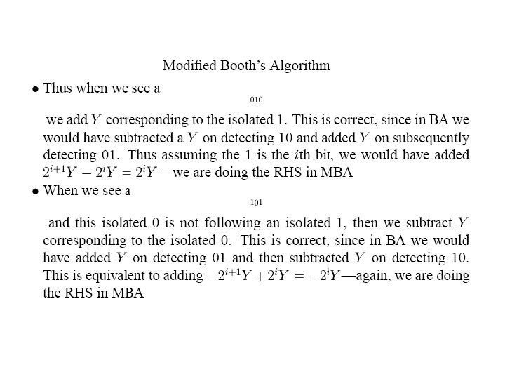
001000

Booth Multiplication Example Multplicand Y = 01001101 = 77, Multiplier X = 11100111 = -25, -Y = 10110011= -77 Cout-AC-Q-q- = 0| 0000 | 11100111 | 0 M = 01001101 (q- is the “prev” bit of Q) Iter 1: q 0 -q- = 10, perform sub AC-Y: 0000 + 10110011 0 10110011 = Cout-AC No ovfl, ASR AC-Q-q-: 11011001 | 11110011 | 1 Iter 2: q 0 -q- = 11, only ASR AC-Q-q-: 11101100 | 11111001 | 1 Iter 3: q 0 -q- = 11, only ASR AC-Q-q-: 11110110 | 01111100 | 1 Iter 4: q 0 -q- = 01, perform add AC+Y: +01001101 1 01000011 = Cout-AC No ovfl, ASR AC-Q-q-: 00100001 | 10111110 | 0 Iter 5: q 0 -q- = 00, only ASR AC-Q-q-: 00010000 | 11011111 | 0 Iter 6: q 0 -q- = 10, perform sub AC-Y: + 10110011 0 11000011 = Cout-AC No ovfl, ASR AC-Q-q-: 11100001 | 11101111 | 1 Iter 7: q 0 -q- = 11, only ASR AC-Q-q-: 11110000 | 11110111 | 1 Iter 8: q 0 -q- = 11, only ASR AC-Q-q-: 11111000 | 01111011 | 1 P = AC-Q = 1111100001111011 = -1925 = 77 x (-25) Needed only 3 +/-’s as opposed to 6 +/-’s needed in regular A&S mult. # of shifts remain the same (8)

Structural VHDL allows the designer to represent a system in terms of components and their interconnections. This module discusses the constructs available in VHDL to facilitate structural descriptions of designs. Acknowledgement (this and next 3 slides): http: //www. people. vcu. edu/~rhklenke/tutorials/vhdl/modules/m 11_23/sld 001. htm. The next 3 slides appear in sld 037. htm to sld 039. htm of this module.

: Structural Description Control signals (from the CU) The final example is of an RTL level datapath for an unsigned 8 bit multiplier. It illustrates the use of complex components in a structural description and the use of multiple levels of hierarchy in that the components are themselves structural descriptions of lower level components. This is the entity description for the datapath. The register controls (enable, mode) will go to the control unit when it is added.

This shows the component declarations and binding indications for the datapath.

scan_out => OPEN, This is the component instantiations for the datapath. The mapping of individual bits of the D and Q input and output of the shift registers is necessary to reverse the inputs and outputs. Recall that the shift register was a “shift up” type where the scan_in input goes to D(0) and D(0) to D(6) go to D(1) to D(7) when in shift mode. What is needed for the multiplier is a “shift down” type register where scan_in goes to D(7), etc. It should have been possible (we believe) to use the syntax d => multiplier(0 to 7) in the shift_reg 8_str PORT MAP to accomplish the same thing, but the Quick. VHDL compiler gave a “warning” and the simulator crashed, so we don’t know if it really should work.

Acknowledgement (this and next 7 slides): http: //www. people. vcu. edu/~rhklenke/tutorials/vhdl/modules/m 12_23/sld 001. htm. The next 7 slides appear in sld 050. htm to sld 056. htm of this module.

: Behavioral Description Now we are going to develop a behavioral description of the controller for the unsigned 8 bit multiplier. This is a flow chart of the algorithm that the controller uses.

This is state diagram of the controller state machine. The outputs for each state aren’t shown for clarity. Notice that there is also a “count” variable that must be included in the state machine to count the number of iterations through the loop. The count variable is actually implemented as another state variable.

The state machine actually has two state variables, the current state of the control state machine (e. g. , initialize, shift, add), and the present loop count. The loop count is a state variable in that it has a present value and a next value, and it is updated in the clock process. However, the value of count only affects the next control state the machine goes to and doesn’t affect the outputs. The implementation is actually more like two state machines in the same architecture.

Control signals (from the CU) This the entity description for the unsigned 8 bit multiplier control unit. It hooks to the datapath via the control signals listed.

This is the beginning of the architecture of the control unit. Note that the constrained subtype of integer is for synthesis - unconstrained integers are hard to synthesize! Also note the state variables are enumerated types. This allows the synthesis tools to encode the state variable using different schemes. Also included here is the clock process. Note that it is edge triggered and that both present_state and present_count are updated on the clock edge. Also note the asynchronous reset signal.

This is the state transition process for the state machine. Note the default assignment of next_state = present_state which is only really required for (some) synthesis tools.

Reset active low x_enable = 1 allows reg. x to be loaded w/ its i/ps: inp. bus or shift inp. x_mode = 1 à load x from inp. bus x_mode = 0 à load x from shift inp. This is the output process. Note that the outputs are only dependent on the present_state variable (Moore machine).