ECE 3317 Applied Electromagnetic Waves Prof David R

ECE 3317 Applied Electromagnetic Waves Prof. David R. Jackson Fall 2020 Notes 8 Transmission Lines (Bounce Diagram) 1

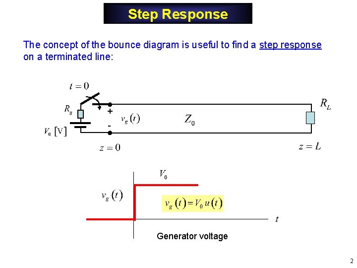
Step Response The concept of the bounce diagram is useful to find a step response on a terminated line: + - Generator voltage 2

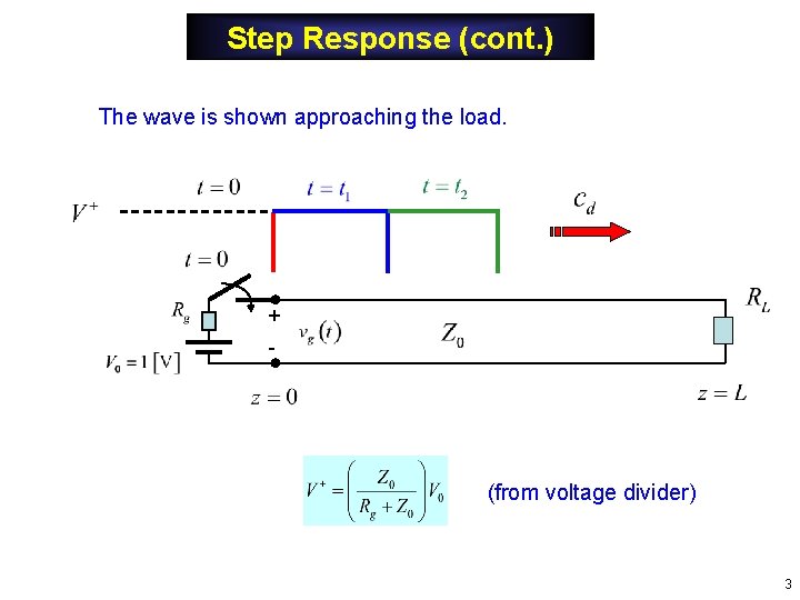
Step Response (cont. ) The wave is shown approaching the load. + - (from voltage divider) 3

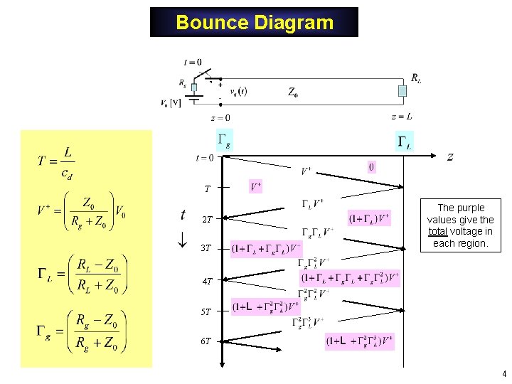
Bounce Diagram T 2 T 3 T The purple values give the total voltage in each region. 4 T 5 T 6 T 4

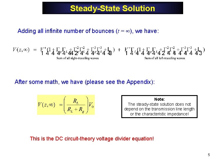
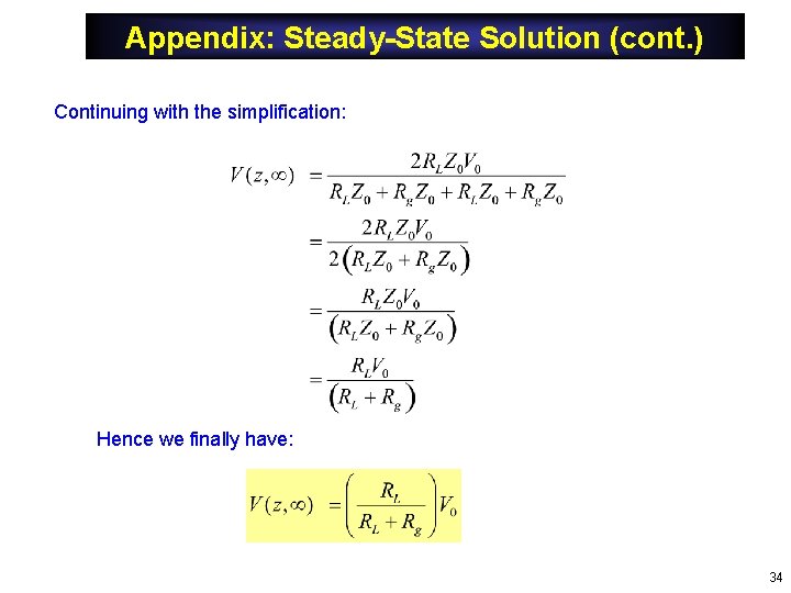
Steady-State Solution Adding all infinite number of bounces (t = ), we have: After some math, we have (please see the Appendix): Note: The steady-state solution does not depend on the transmission line length or the characteristic impedance! This is the DC circuit-theory voltage divider equation! 5

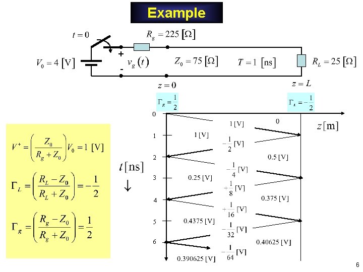
Example + - 1 2 3 4 5 6 6

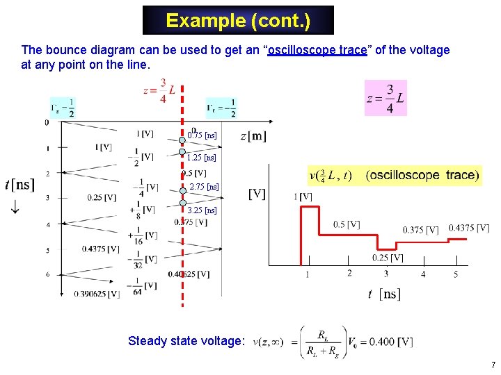
Example (cont. ) The bounce diagram can be used to get an “oscilloscope trace” of the voltage at any point on the line. 0. 75 [ns] 1. 25 [ns] 2. 75 [ns] 3. 25 [ns] Steady state voltage: 7

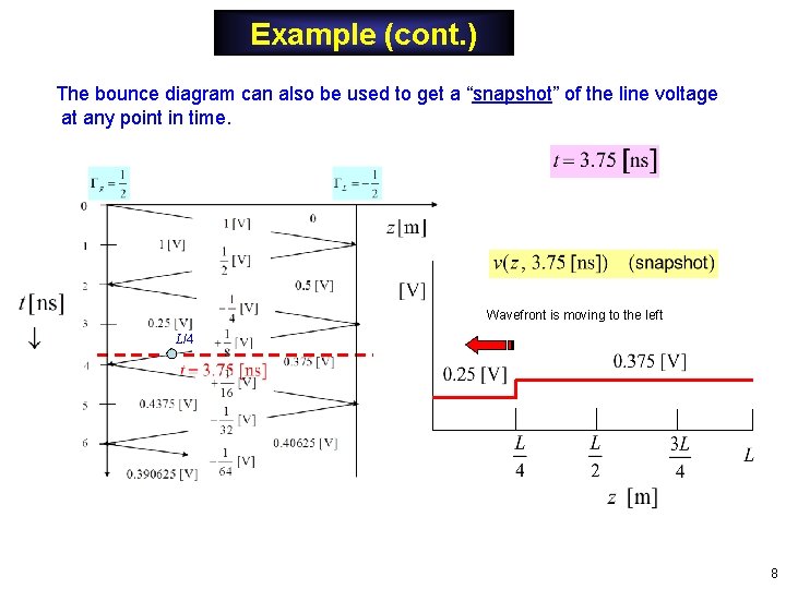
Example (cont. ) The bounce diagram can also be used to get a “snapshot” of the line voltage at any point in time. Wavefront is moving to the left L/4 8

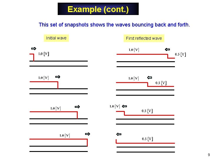
Example (cont. ) This set of snapshots shows the waves bouncing back and forth. Initial wave First reflected wave 9

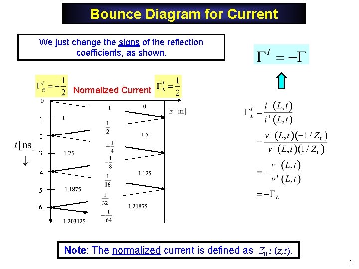
Bounce Diagram for Current We just change the signs of the reflection coefficients, as shown. Normalized Current 1 2 3 4 5 6 Note: The normalized current is defined as Z 0 i (z, t). 10

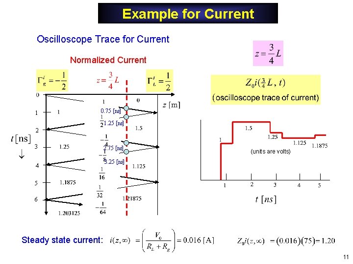
Example for Current Oscilloscope Trace for Current Normalized Current 1 0. 75 [ns] 1. 25 [ns] 2 3 4 2. 75 [ns] (units are volts) 3. 25 [ns] 5 6 Steady state current: 11

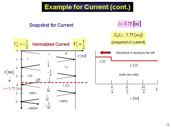
Example for Current (cont. ) Snapshot for Current Normalized Current Wavefront is moving to the left 1 2 (units are volts) 3 L/4 4 5 6 12

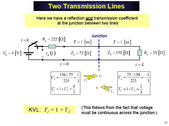
Two Transmission Lines Here we have a reflection and transmission coefficient at the junction between two lines Junction + - KVL: TJ = 1 + J (This follows from the fact that voltage must be continuous across the junction. ) 13

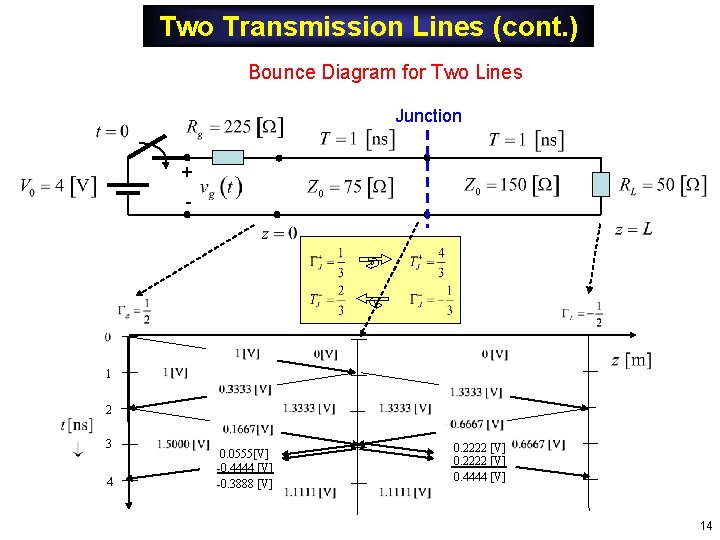
Two Transmission Lines (cont. ) Bounce Diagram for Two Lines Junction + - 1 2 3 4 0. 0555[V] -0. 4444 [V] -0. 3888 [V] 0. 2222 [V] 0. 4444 [V] 14

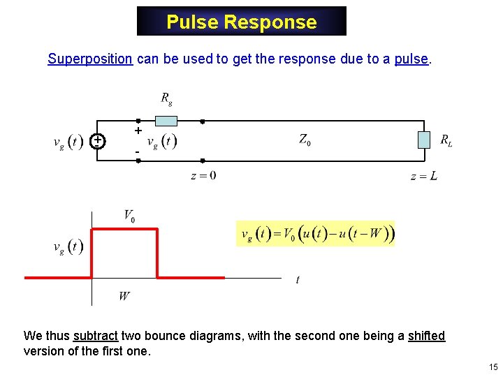
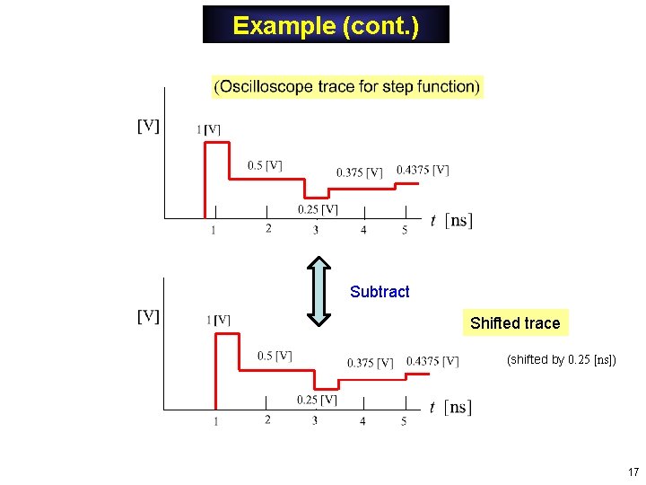
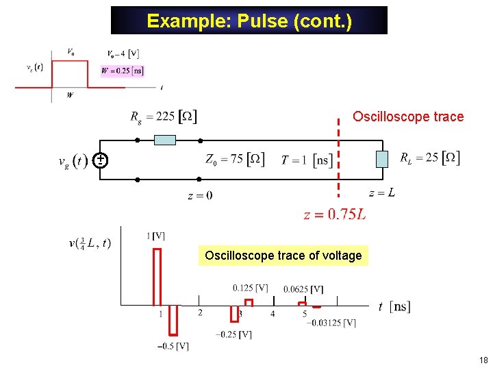
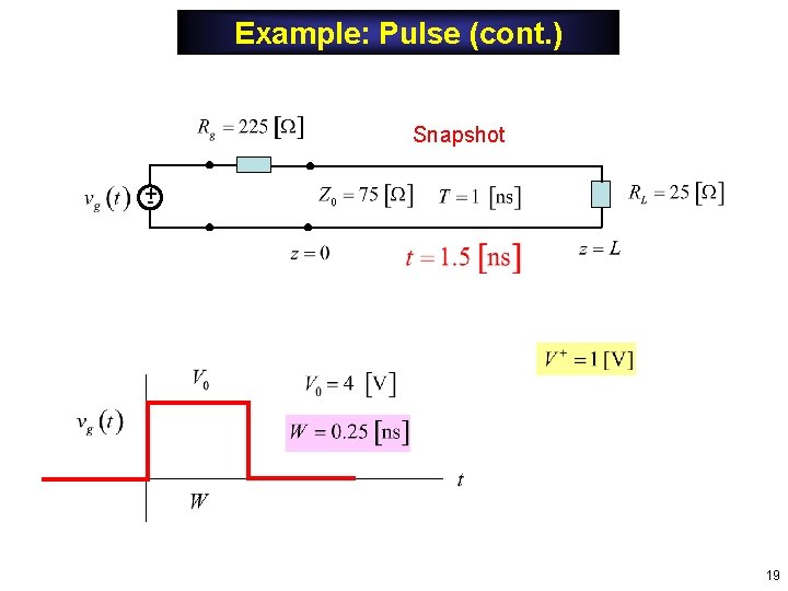
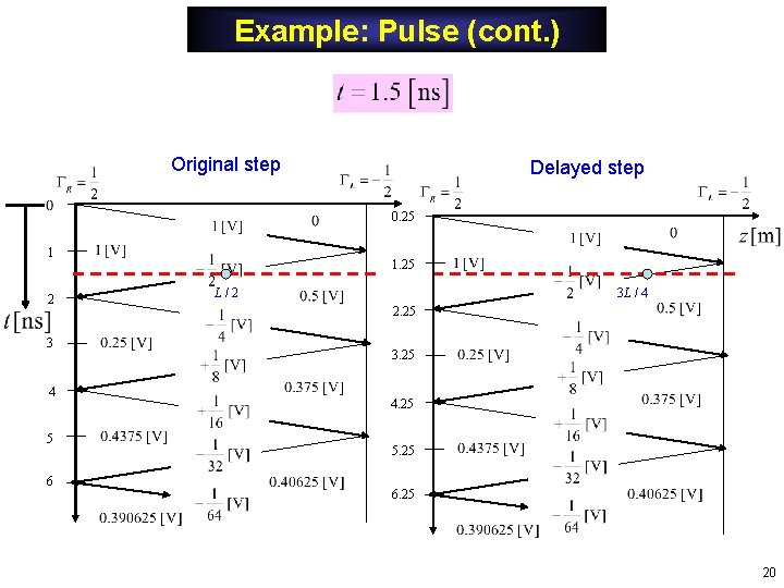
Pulse Response Superposition can be used to get the response due to a pulse. +- + - We thus subtract two bounce diagrams, with the second one being a shifted version of the first one. 15

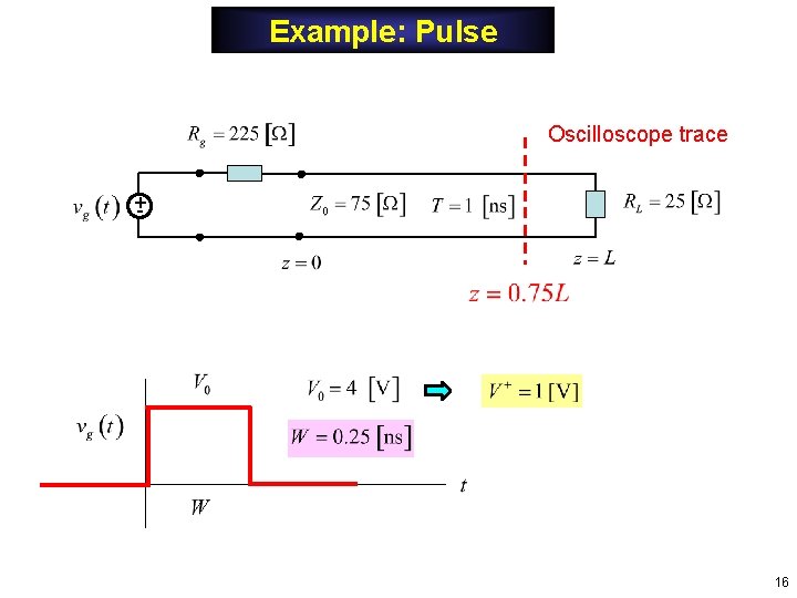
Example: Pulse Oscilloscope trace +- 16

Example (cont. ) Subtract Shifted trace (shifted by 0. 25 [ns]) 17

Example: Pulse (cont. ) Oscilloscope trace +- Oscilloscope trace of voltage 18

Example: Pulse (cont. ) Snapshot +- 19

Example: Pulse (cont. ) Original step Delayed step 0. 25 1 2 3 4 5 6 1. 25 L/2 3 L / 4 2. 25 3. 25 4. 25 5. 25 6. 25 20

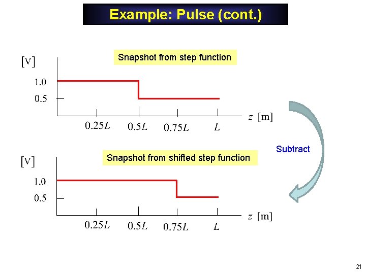
Example: Pulse (cont. ) Snapshot from step function Snapshot from shifted step function Subtract 21

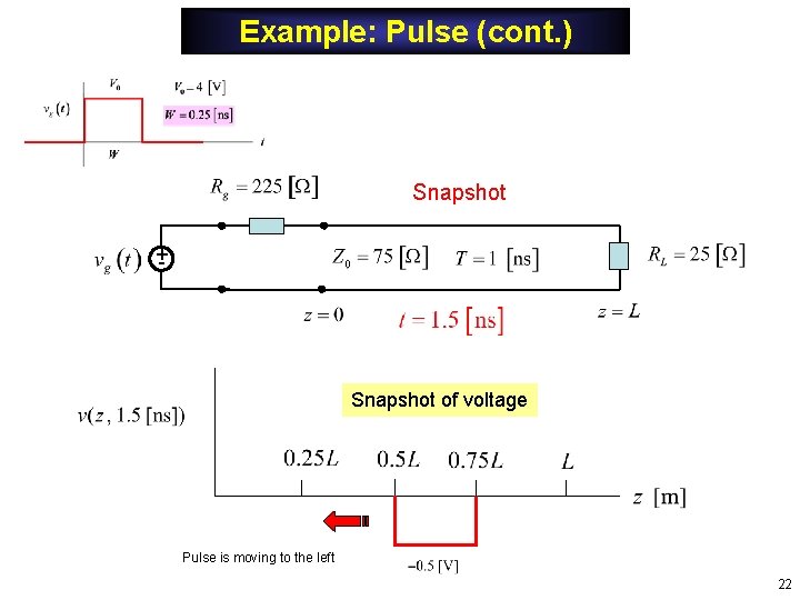
Example: Pulse (cont. ) Snapshot +- Snapshot of voltage Pulse is moving to the left 22

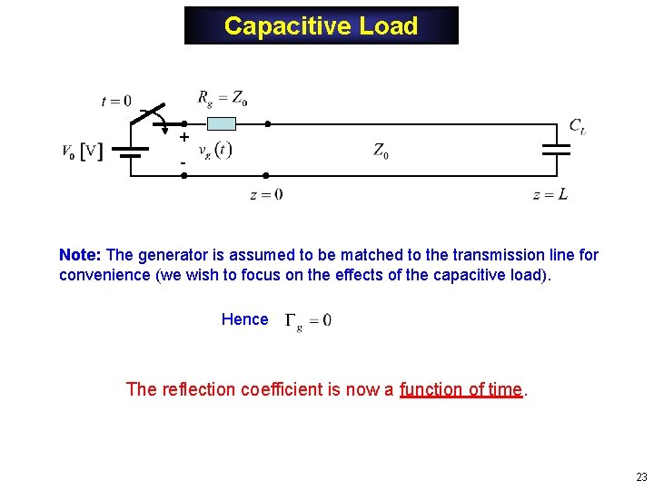
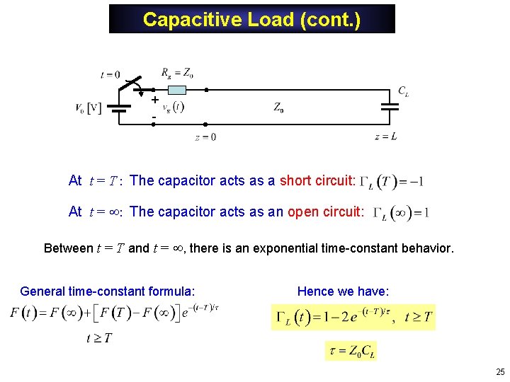
Capacitive Load + - Note: The generator is assumed to be matched to the transmission line for convenience (we wish to focus on the effects of the capacitive load). Hence The reflection coefficient is now a function of time. 23

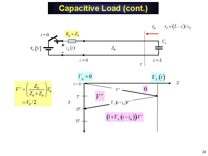
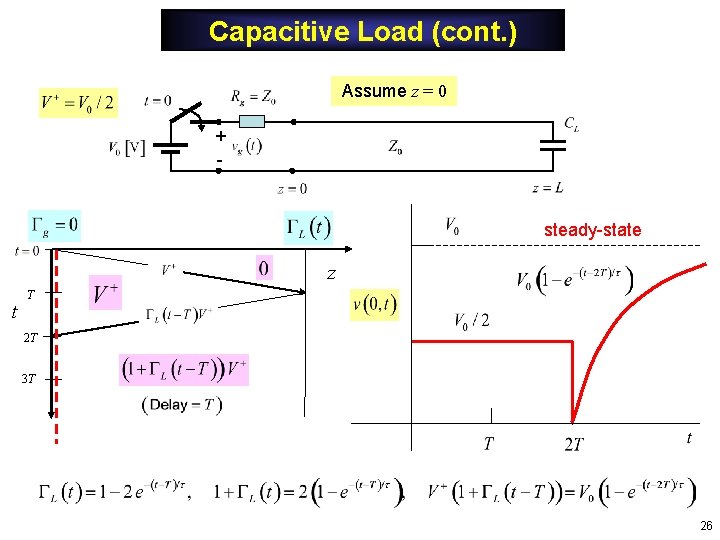
Capacitive Load (cont. ) + - z T t 2 T 3 T 24

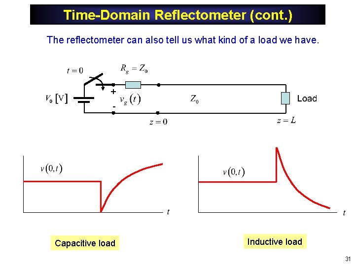
Capacitive Load (cont. ) + - At t = T : The capacitor acts as a short circuit: At t = : The capacitor acts as an open circuit: Between t = T and t = , there is an exponential time-constant behavior. General time-constant formula: Hence we have: 25

Capacitive Load (cont. ) Assume z = 0 + - steady-state z t T 2 T 3 T 26

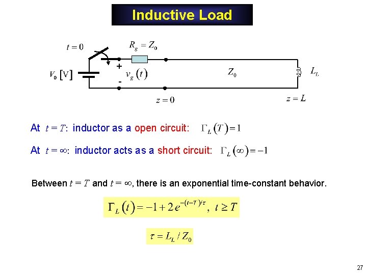
Inductive Load + - At t = T: inductor as a open circuit: At t = : inductor acts as a short circuit: Between t = T and t = , there is an exponential time-constant behavior. 27

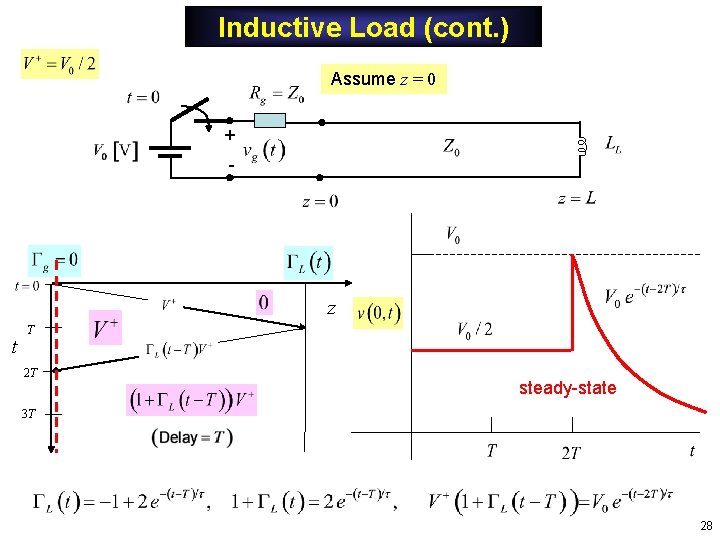
Inductive Load (cont. ) Assume z = 0 + - z t T 2 T steady-state 3 T 28

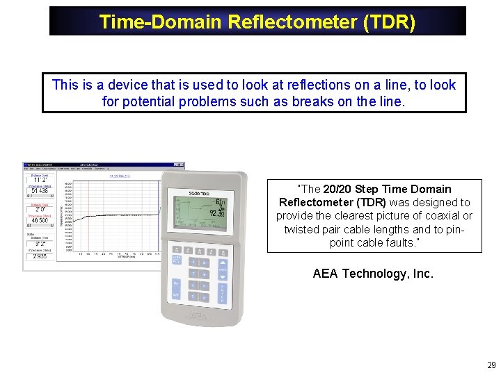
Time-Domain Reflectometer (TDR) This is a device that is used to look at reflections on a line, to look for potential problems such as breaks on the line. “The 20/20 Step Time Domain Reflectometer (TDR) was designed to provide the clearest picture of coaxial or twisted pair cable lengths and to pinpoint cable faults. ” AEA Technology, Inc. 29

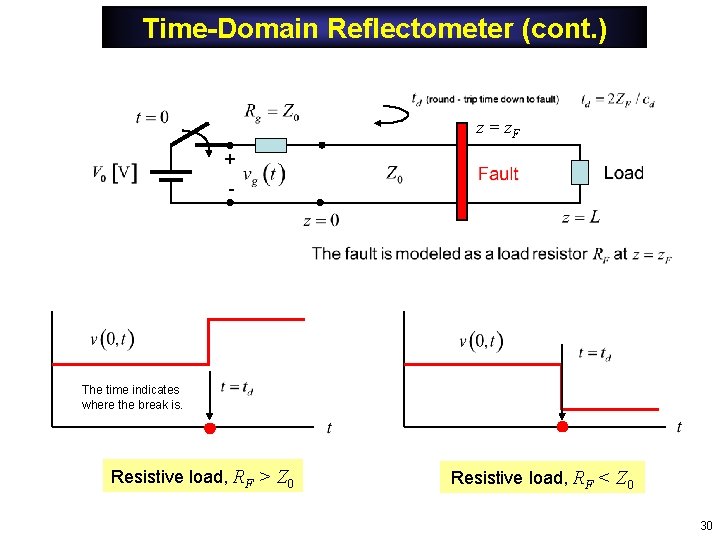
Time-Domain Reflectometer (cont. ) z = z. F + - The time indicates where the break is. Resistive load, RF > Z 0 Resistive load, RF < Z 0 30

Time-Domain Reflectometer (cont. ) The reflectometer can also tell us what kind of a load we have. + - Capacitive load Inductive load 31

Appendix: Steady-State Solution Adding all infinite number of bounces (t = ), we have: Note: We have used 32

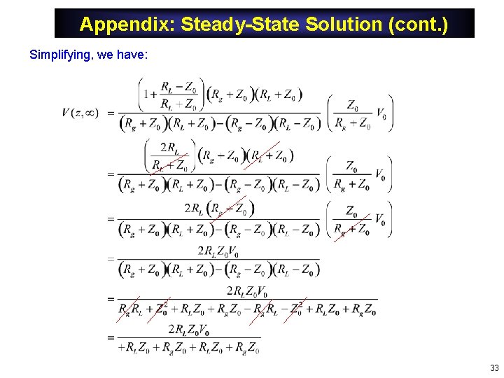
Appendix: Steady-State Solution (cont. ) Simplifying, we have: 33

Appendix: Steady-State Solution (cont. ) Continuing with the simplification: Hence we finally have: 34