ECE 3317 Applied Electromagnetic Waves Prof David R

ECE 3317 Applied Electromagnetic Waves Prof. David R. Jackson Fall 2018 Notes 20 Rectangular Waveguides 1

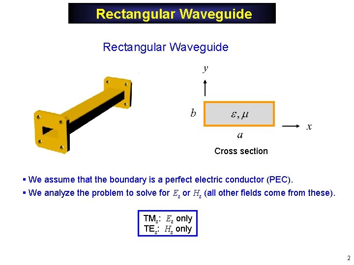
Rectangular Waveguide Cross section § We assume that the boundary is a perfect electric conductor (PEC). § We analyze the problem to solve for Ez or Hz (all other fields come from these). TMz: Ez only TEz: Hz only 2

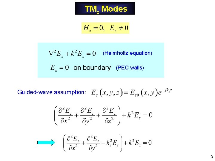
TMz Modes (Helmholtz equation) (PEC walls) Guided-wave assumption: 3

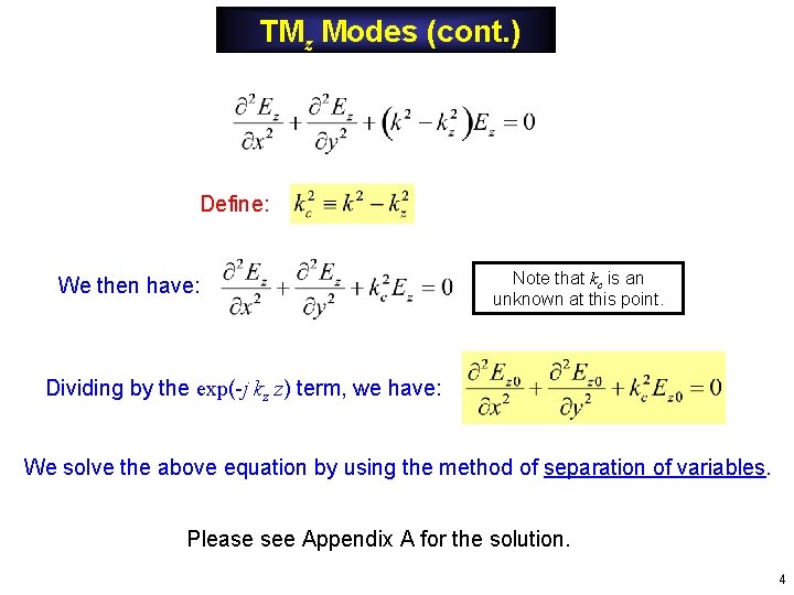
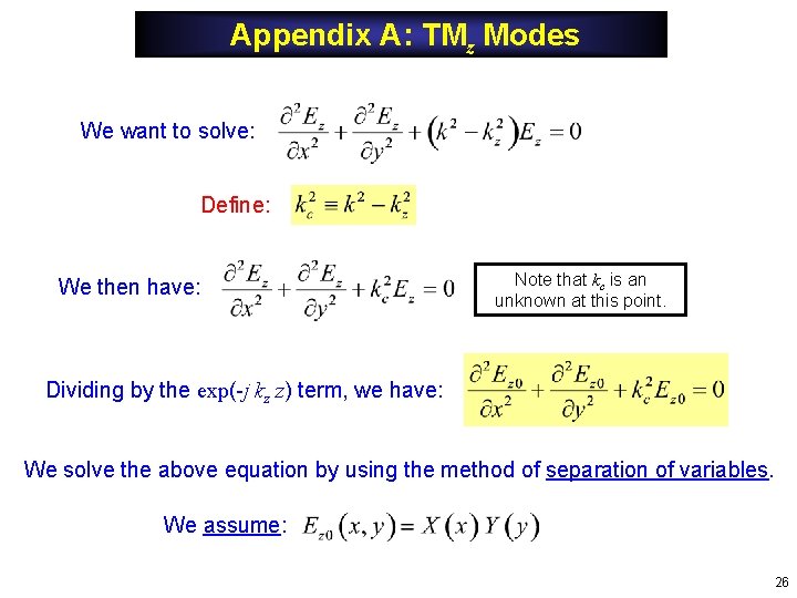
TMz Modes (cont. ) Define: We then have: Note that kc is an unknown at this point. Dividing by the exp(-j kz z) term, we have: We solve the above equation by using the method of separation of variables. Please see Appendix A for the solution. 4

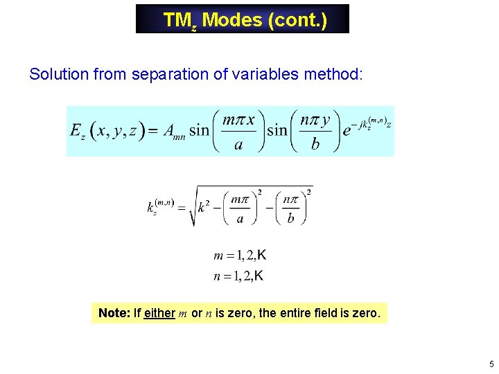
TMz Modes (cont. ) Solution from separation of variables method: Note: If either m or n is zero, the entire field is zero. 5

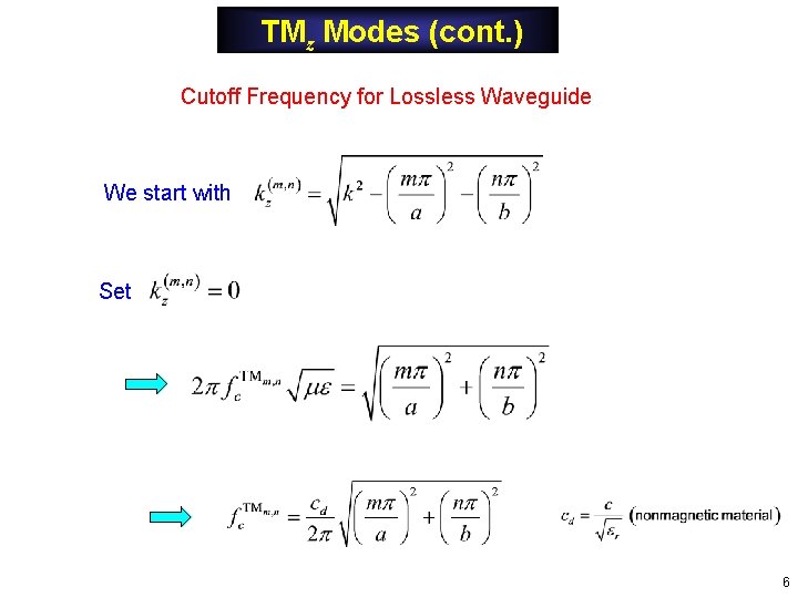
TMz Modes (cont. ) Cutoff Frequency for Lossless Waveguide We start with Set 6

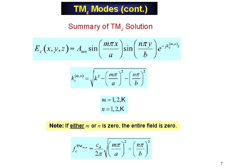
TMz Modes (cont. ) Summary of TMz Solution Note: If either m or n is zero, the entire field is zero. 7

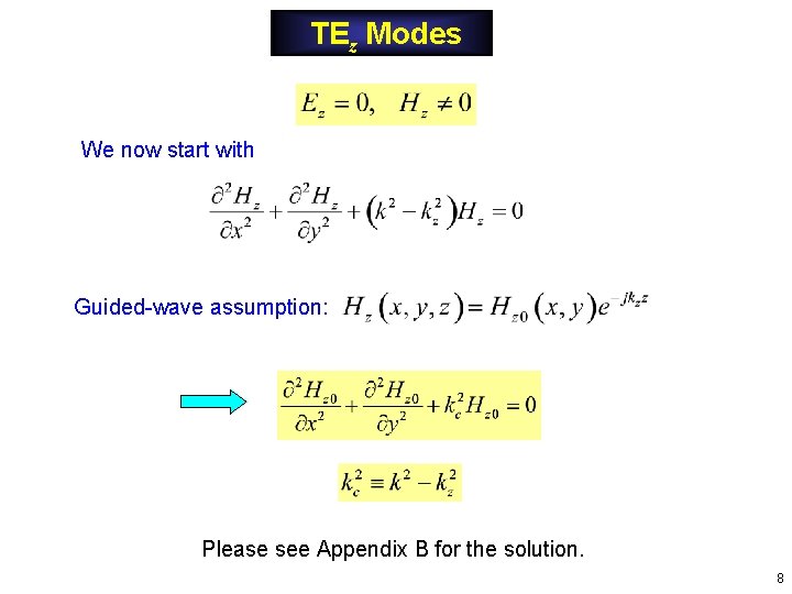
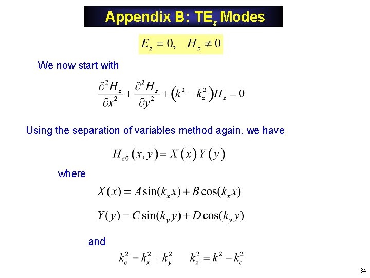
TEz Modes We now start with Guided-wave assumption: Please see Appendix B for the solution. 8

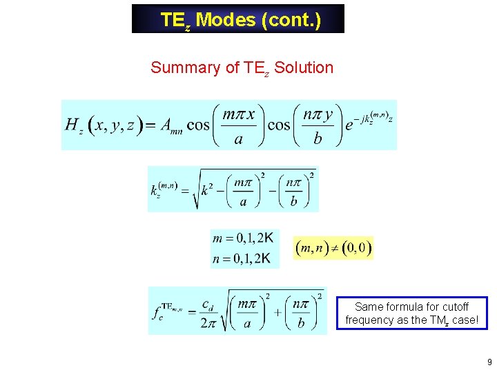
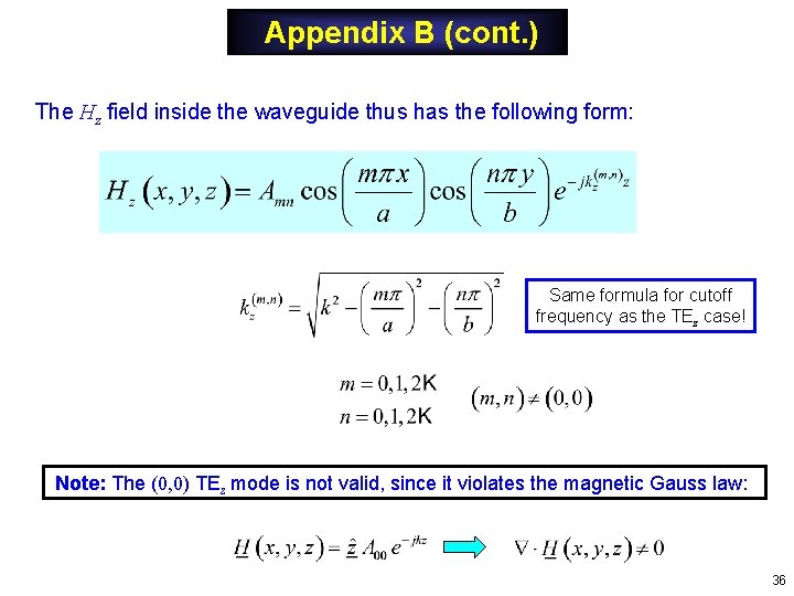
TEz Modes (cont. ) Summary of TEz Solution Same formula for cutoff frequency as the TMz case! 9

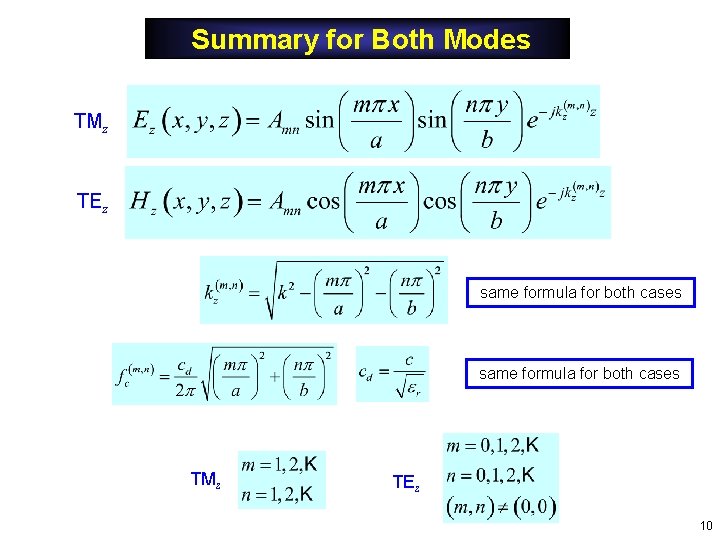
Summary for Both Modes TMz TEz same formula for both cases TMz TEz 10

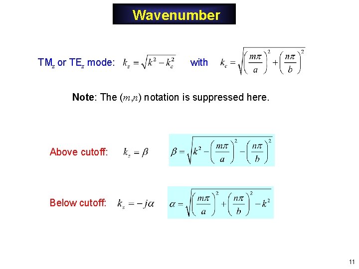
Wavenumber TMz or TEz mode: with Note: The (m, n) notation is suppressed here. Above cutoff: Below cutoff: 11

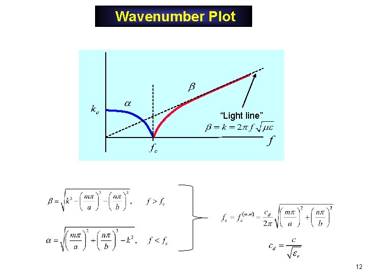
Wavenumber Plot “Light line” 12

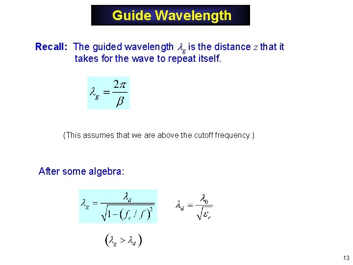
Guide Wavelength Recall: The guided wavelength g is the distance z that it takes for the wave to repeat itself. (This assumes that we are above the cutoff frequency. ) After some algebra: 13

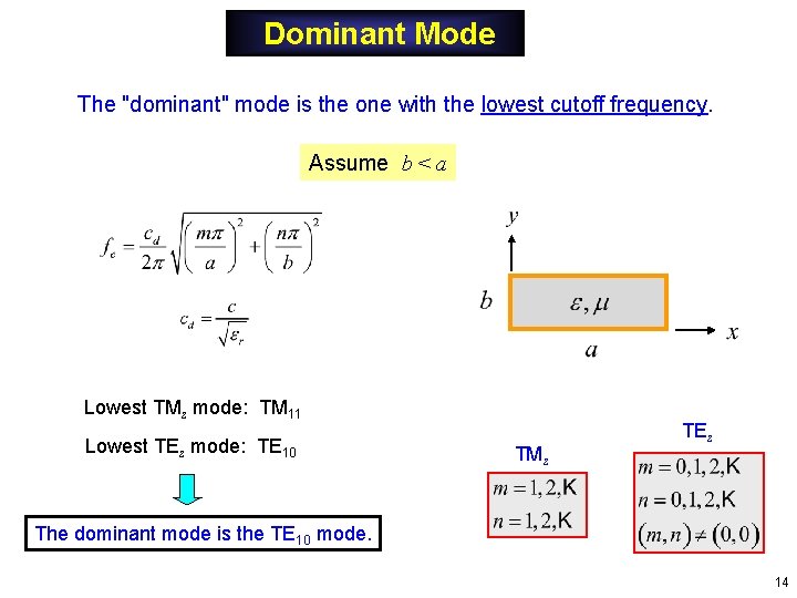
Dominant Mode The "dominant" mode is the one with the lowest cutoff frequency. Assume b < a Lowest TMz mode: TM 11 Lowest TEz mode: TE 10 TMz TEz The dominant mode is the TE 10 mode. 14

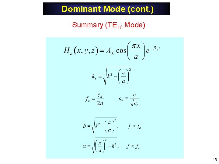
Dominant Mode (cont. ) Summary (TE 10 Mode) 15

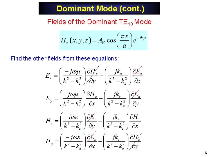
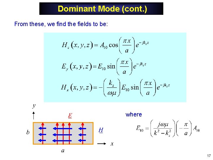
Dominant Mode (cont. ) Fields of the Dominant TE 10 Mode Find the other fields from these equations: 16

Dominant Mode (cont. ) From these, we find the fields to be: where 17

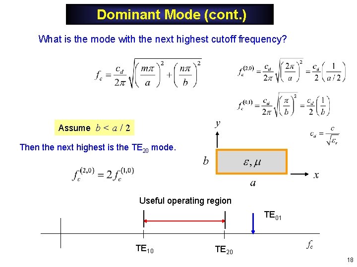
Dominant Mode (cont. ) What is the mode with the next highest cutoff frequency? Assume b < a / 2 Then the next highest is the TE 20 mode. Useful operating region TE 01 TE 10 TE 20 fc 18

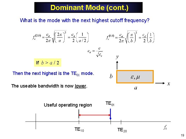
Dominant Mode (cont. ) What is the mode with the next highest cutoff frequency? If b > a / 2 Then the next highest is the TE 01 mode. The useable bandwidth is now lower. Useful operating region TE 10 TE 01 TE 20 fc 19

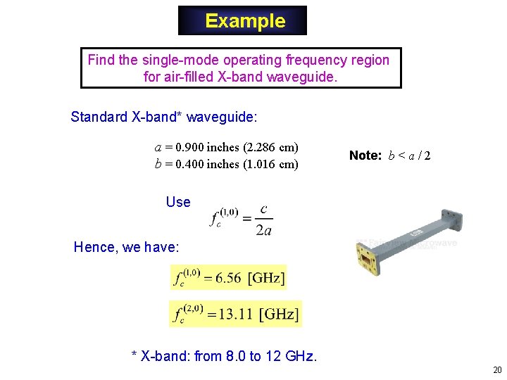
Example Find the single-mode operating frequency region for air-filled X-band waveguide. Standard X-band* waveguide: a = 0. 900 inches (2. 286 cm) b = 0. 400 inches (1. 016 cm) Note: b < a / 2 Use Hence, we have: * X-band: from 8. 0 to 12 GHz. 20

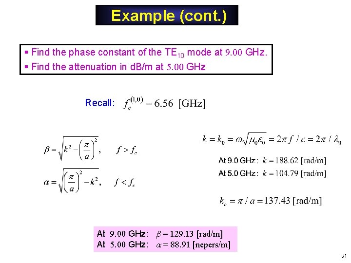
Example (cont. ) § Find the phase constant of the TE 10 mode at 9. 00 GHz. § Find the attenuation in d. B/m at 5. 00 GHz Recall: At 9. 00 GHz: = 129. 13 [rad/m] At 5. 00 GHz: = 88. 91 [nepers/m] 21

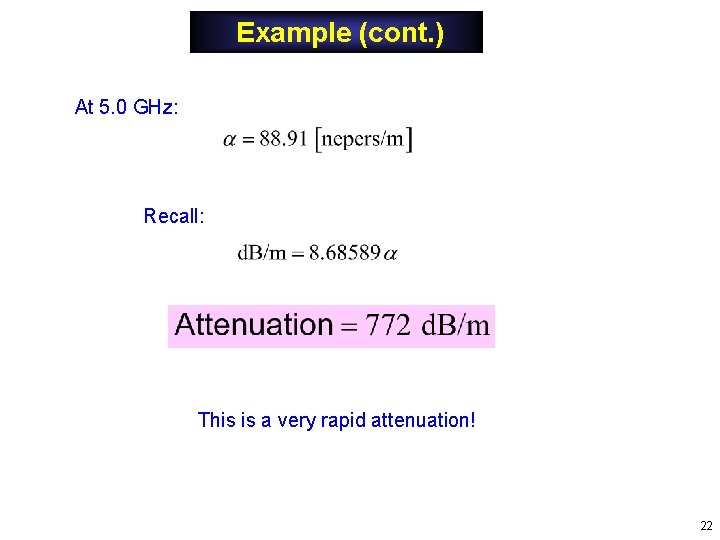
Example (cont. ) At 5. 0 GHz: Recall: This is a very rapid attenuation! 22

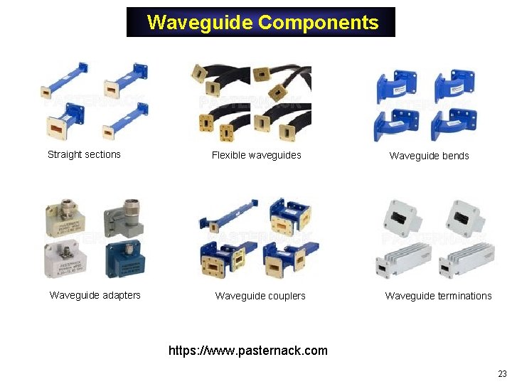
Waveguide Components Straight sections Waveguide adapters Flexible waveguides Waveguide couplers Waveguide bends Waveguide terminations https: //www. pasternack. com 23

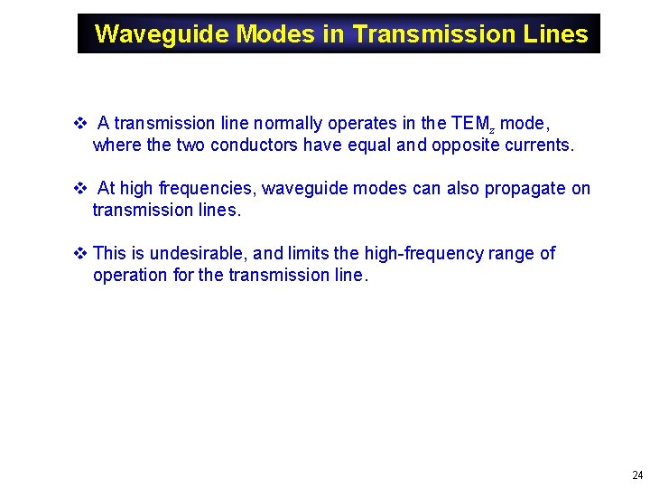
Waveguide Modes in Transmission Lines v A transmission line normally operates in the TEMz mode, where the two conductors have equal and opposite currents. v At high frequencies, waveguide modes can also propagate on transmission lines. v This is undesirable, and limits the high-frequency range of operation for the transmission line. 24

Waveguide Modes in Coax Dominant waveguide mode in coax (derivation omitted): TE 11 mode Example: RG 142 coax 25

Appendix A: TMz Modes We want to solve: Define: We then have: Note that kc is an unknown at this point. Dividing by the exp(-j kz z) term, we have: We solve the above equation by using the method of separation of variables. We assume: 26

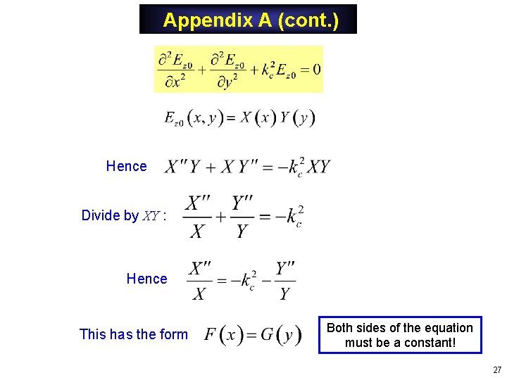
Appendix A (cont. ) Hence Divide by XY : Hence This has the form Both sides of the equation must be a constant! 27

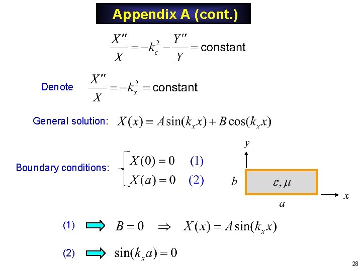
Appendix A (cont. ) Denote General solution: Boundary conditions: (1) (2) 28

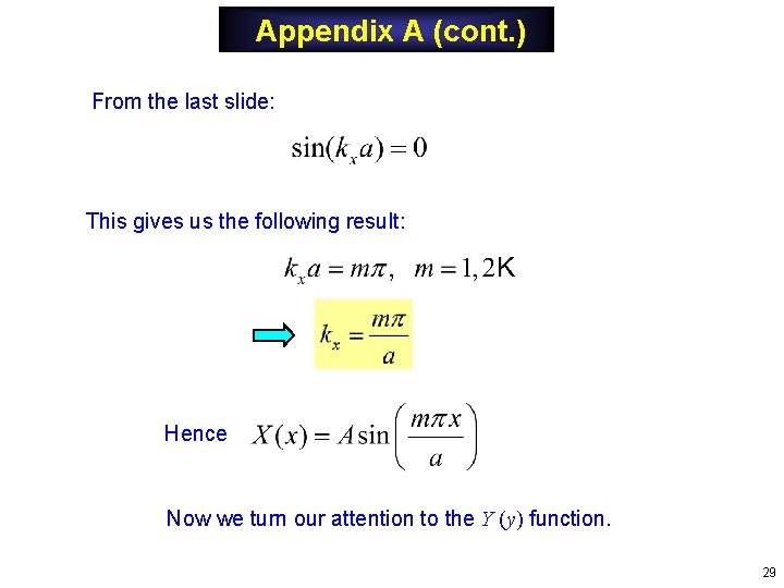
Appendix A (cont. ) From the last slide: This gives us the following result: Hence Now we turn our attention to the Y (y) function. 29

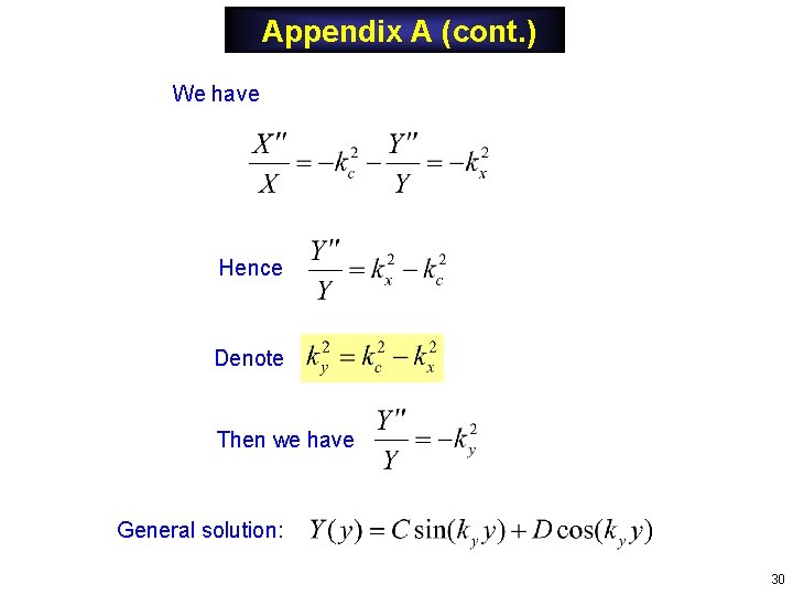
Appendix A (cont. ) We have Hence Denote Then we have General solution: 30

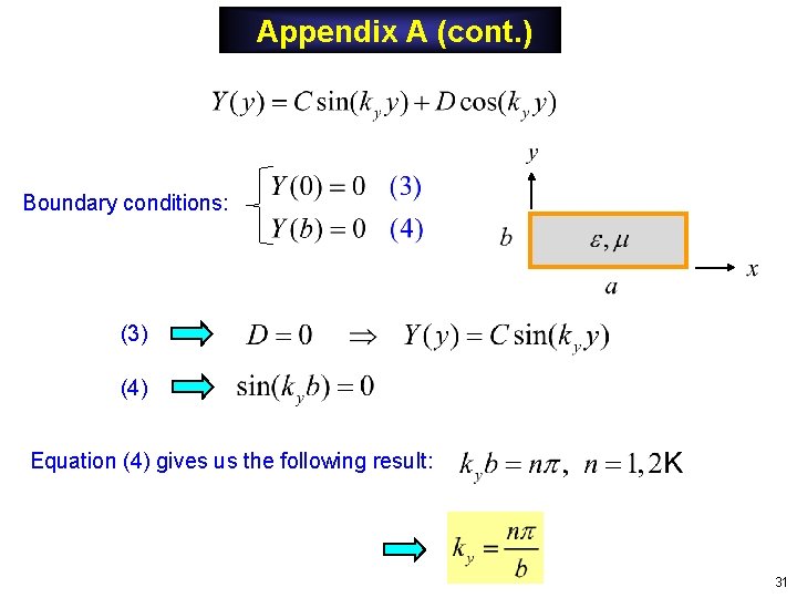
Appendix A (cont. ) Boundary conditions: (3) (4) Equation (4) gives us the following result: 31

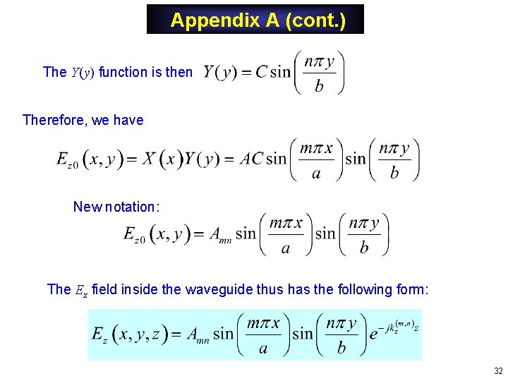
Appendix A (cont. ) The Y(y) function is then Therefore, we have New notation: The Ez field inside the waveguide thus has the following form: 32

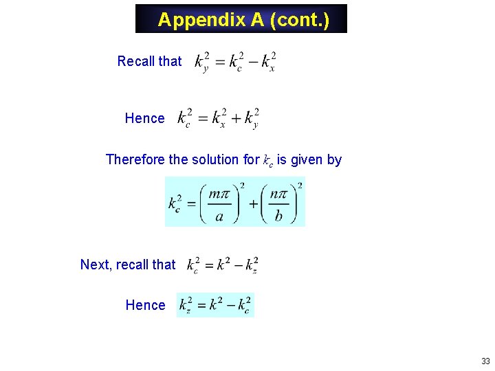
Appendix A (cont. ) Recall that Hence Therefore the solution for kc is given by Next, recall that Hence 33

Appendix B: TEz Modes We now start with Using the separation of variables method again, we have where and 34

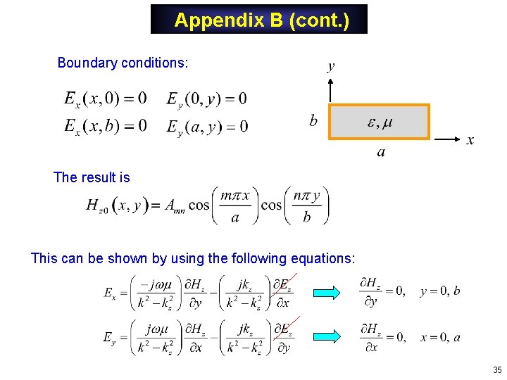
Appendix B (cont. ) Boundary conditions: The result is This can be shown by using the following equations: 35

Appendix B (cont. ) The Hz field inside the waveguide thus has the following form: Same formula for cutoff frequency as the TEz case! Note: The (0, 0) TEz mode is not valid, since it violates the magnetic Gauss law: 36