ECE 3163 8443Signals Pattern and Recognition ECE Systems

ECE 3163 8443––Signals Pattern and Recognition ECE Systems LECTURE 20: FOURIER ANALYSIS OF DT SYSTEMS • Objectives: Frequency Response of a Sinusoid DT MA Filter Design DT WMA Filter • Resources: Wiki: Fourier Analysis Wiki: Moving Average USU: The Discrete-Time FT DSPGuide: Moving Average Filters Logix 4 u: MA Demo • URL: . . . /publications/courses/ece_3163/lectures/current/lecture_20. ppt • MP 3: . . . /publications/courses/ece_3163/lectures/current/lecture_20. mp 3

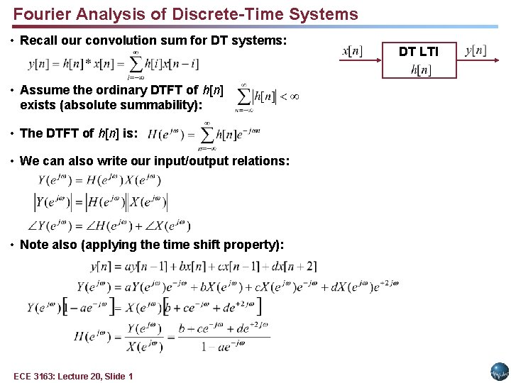
Fourier Analysis of Discrete-Time Systems • Recall our convolution sum for DT systems: • Assume the ordinary DTFT of h[n] exists (absolute summability): • The DTFT of h[n] is: • We can also write our input/output relations: • Note also (applying the time shift property): ECE 3163: Lecture 20, Slide 1 DT LTI

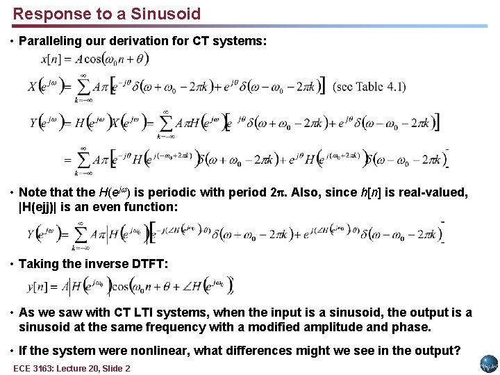
Response to a Sinusoid • Paralleling our derivation for CT systems: • Note that the H(ej ) is periodic with period 2. Also, since h[n] is real-valued, |H(ejj)| is an even function: • Taking the inverse DTFT: • As we saw with CT LTI systems, when the input is a sinusoid, the output is a sinusoid at the same frequency with a modified amplitude and phase. • If the system were nonlinear, what differences might we see in the output? ECE 3163: Lecture 20, Slide 2

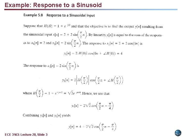
Example: Response to a Sinusoid ECE 3163: Lecture 20, Slide 3

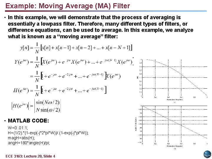
Example: Moving Average (MA) Filter • In this example, we will demonstrate that the process of averaging is essentially a lowpass filter. Therefore, many different types of filters, or difference equations, can be used to average. In this example, we analyze what is known as a “moving average” filter: • MATLAB CODE: W=0: . 01: 1; H=(1/2). *(1 -exp(-j*2*pi*W))/. (1 -exp(-j*pi*W)); mag. H=abs(H); ang. H=180*angle(H)/pi; ECE 3163: Lecture 20, Slide 4

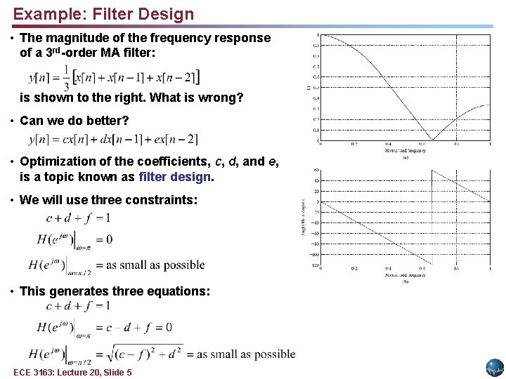
Example: Filter Design • The magnitude of the frequency response of a 3 rd-order MA filter: is shown to the right. What is wrong? • Can we do better? • Optimization of the coefficients, c, d, and e, is a topic known as filter design. • We will use three constraints: • This generates three equations: ECE 3163: Lecture 20, Slide 5

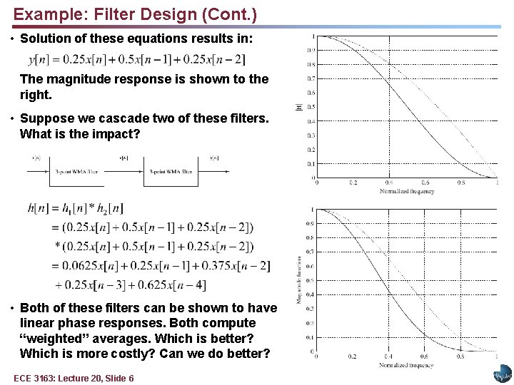
Example: Filter Design (Cont. ) • Solution of these equations results in: The magnitude response is shown to the right. • Suppose we cascade two of these filters. What is the impact? • Both of these filters can be shown to have linear phase responses. Both compute “weighted” averages. Which is better? Which is more costly? Can we do better? ECE 3163: Lecture 20, Slide 6

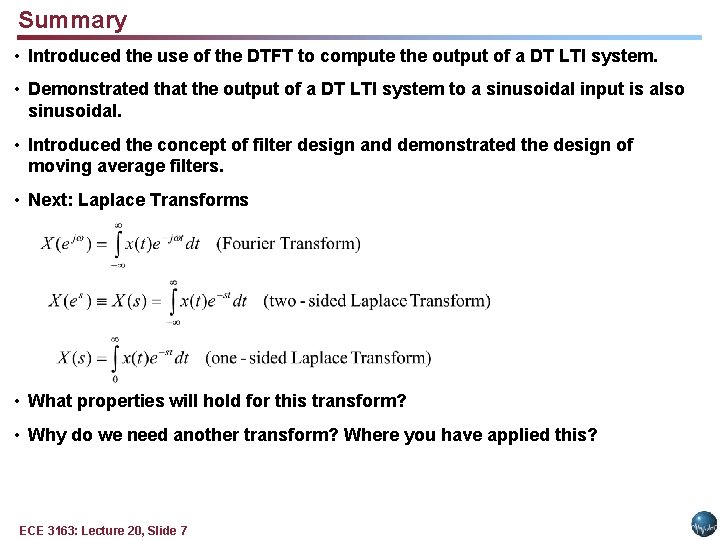
Summary • Introduced the use of the DTFT to compute the output of a DT LTI system. • Demonstrated that the output of a DT LTI system to a sinusoidal input is also sinusoidal. • Introduced the concept of filter design and demonstrated the design of moving average filters. • Next: Laplace Transforms • What properties will hold for this transform? • Why do we need another transform? Where you have applied this? ECE 3163: Lecture 20, Slide 7