ECE 2795 Microgrid Concepts and Distributed Generation Technologies

ECE 2795 Microgrid Concepts and Distributed Generation Technologies Spring 2015 Week #2 © A. Kwasinski, 2014

Photovoltaic modules • Photovoltaic (PV) modules are made by connecting several PV cells. PV arrays are made by connecting several PV modules. • Although the sun will eventually die as a white dwarf star in about 4. 5 Billion years, solar power can be considered a renewable source of energy because we can expect that for the next couple of billion years the sun will still radiate power without making the Earth inhabitable. • Solar power is radiated through space. • Solar power is generated by nuclear fusion. • Light propagation can be represented through waves or through particles (dual representation). • To represent electricity production in PV cells, the particle (photon) representation is used © A. Kwasinski, 2014

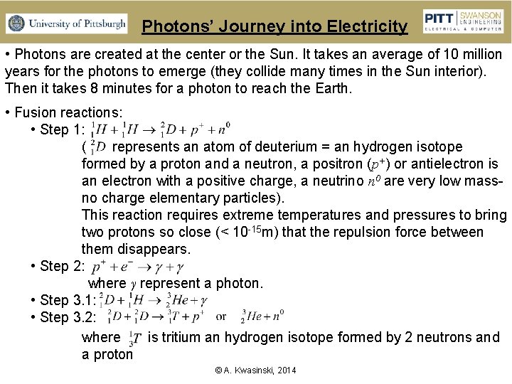
Photons’ Journey into Electricity • Photons are created at the center or the Sun. It takes an average of 10 million years for the photons to emerge (they collide many times in the Sun interior). Then it takes 8 minutes for a photon to reach the Earth. • Fusion reactions: • Step 1: ( represents an atom of deuterium = an hydrogen isotope formed by a proton and a neutron, a positron (p+) or antielectron is an electron with a positive charge, a neutrino n 0 are very low massno charge elementary particles). This reaction requires extreme temperatures and pressures to bring two protons so close (< 10 -15 m) that the repulsion force between them disappears. • Step 2: where γ represent a photon. • Step 3. 1: • Step 3. 2: where is tritium an hydrogen isotope formed by 2 neutrons and a proton © A. Kwasinski, 2014

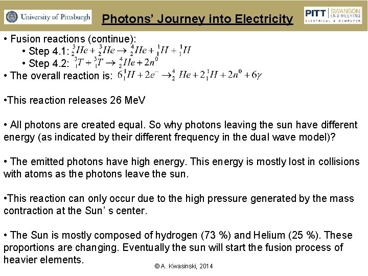
Photons’ Journey into Electricity • Fusion reactions (continue): • Step 4. 1: • Step 4. 2: • The overall reaction is: • This reaction releases 26 Me. V • All photons are created equal. So why photons leaving the sun have different energy (as indicated by their different frequency in the dual wave model)? • The emitted photons have high energy. This energy is mostly lost in collisions with atoms as the photons leave the sun. • This reaction can only occur due to the high pressure generated by the mass contraction at the Sun’ s center. • The Sun is mostly composed of hydrogen (73 %) and Helium (25 %). These proportions are changing. Eventually the sun will start the fusion process of heavier elements. © A. Kwasinski, 2014

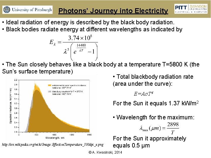
Photons’ Journey into Electricity • Ideal radiation of energy is described by the black body radiation. • Black bodies radiate energy at different wavelengths as indicated by • The Sun closely behaves like a black body at a temperature T=5800 K (the Sun’s surface temperature) • Total blackbody radiation rate (area under the curve): E=AσT 4 For the Sun it equals 1. 37 k. W/m 2 • Wavelength for the maximum: http: //en. wikipedia. org/wiki/Image: Effective. Temperature_300 dpi_e. png For the Sun it approximately equals 0. 5 μm © A. Kwasinski, 2014

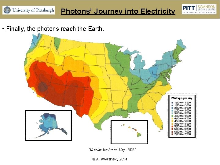
Photons’ Journey into Electricity • Finally, the photons reach the Earth. US Solar Insolation Map: NREL © A. Kwasinski, 2014

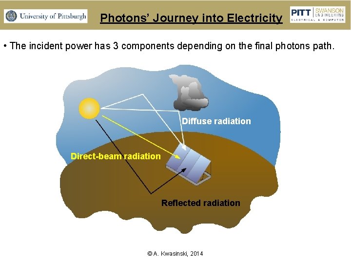
Photons’ Journey into Electricity • The incident power has 3 components depending on the final photons path. Diffuse radiation Direct-beam radiation Reflected radiation © A. Kwasinski, 2014

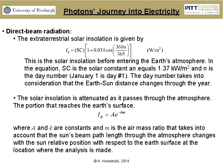
Photons’ Journey into Electricity • Direct-beam radiation: • The extraterrestrial solar insolation is given by This is the solar insolation before entering the Earth’s atmosphere. In the equation, SC is the solar constant an equals 1. 37 k. W/m 2 and n is the day number (January 1 is day #1). The day number takes into consideration that the Earth-Sun distance changes through the year. • The solar insolation is attenuated as it passes through the atmosphere. The portion that reaches the earth’s surface. where A and k are constants and m is the air mass ratio that takes into account that the sun’s beam path length through the atmosphere changes with the sun relative position with respect to the earth surface at the location where the analysis is made. © A. Kwasinski, 2014

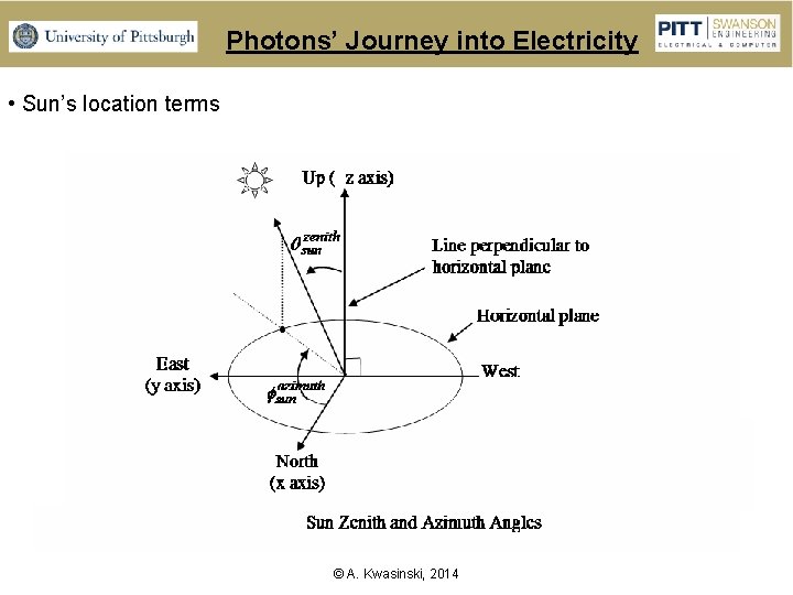
Photons’ Journey into Electricity • Sun’s location terms © A. Kwasinski, 2014

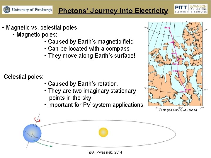
Photons’ Journey into Electricity • Magnetic vs. celestial poles: • Magnetic poles: • Caused by Earth’s magnetic field • Can be located with a compass • They move along Earth’s surface! Celestial poles: • Caused by Earth’s rotation. • They are two imaginary stationary points in the sky. • Important for PV system applications. Geological Survey of Canada © A. Kwasinski, 2014

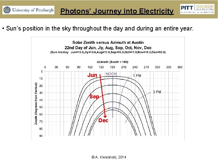
Photons’ Journey into Electricity • Sun’s position in the sky throughout the day and during an entire year. NOON Jun Sep Dec © A. Kwasinski, 2014 1 PM 3 PM

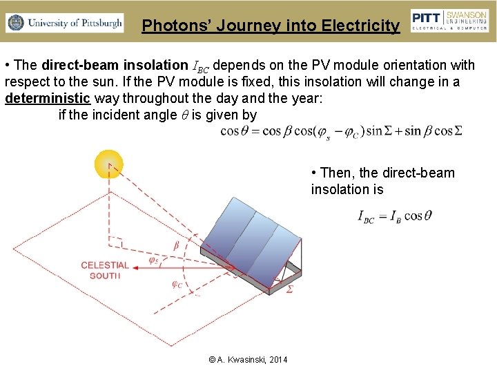
Photons’ Journey into Electricity • The direct-beam insolation IBC depends on the PV module orientation with respect to the sun. If the PV module is fixed, this insolation will change in a deterministic way throughout the day and the year: if the incident angle θ is given by • Then, the direct-beam insolation is © A. Kwasinski, 2014

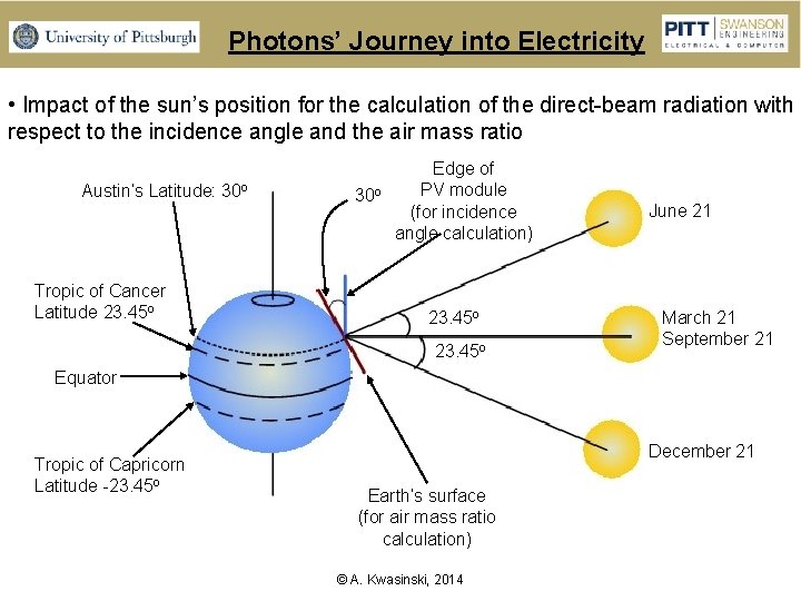
Photons’ Journey into Electricity • Impact of the sun’s position for the calculation of the direct-beam radiation with respect to the incidence angle and the air mass ratio Austin’s Latitude: 30 o Tropic of Cancer Latitude 23. 45 o 30 o Edge of PV module (for incidence angle calculation) 23. 45 o June 21 March 21 September 21 Equator Tropic of Capricorn Latitude -23. 45 o December 21 Earth’s surface (for air mass ratio calculation) © A. Kwasinski, 2014

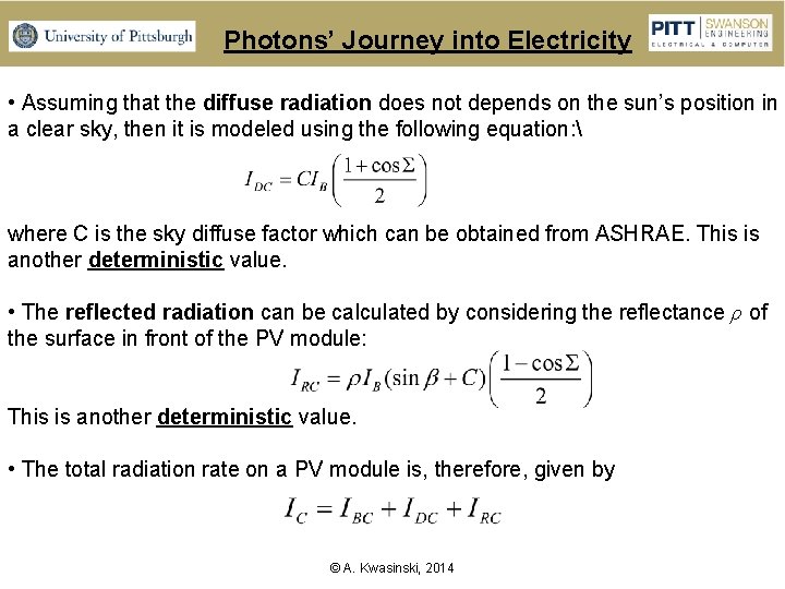
Photons’ Journey into Electricity • Assuming that the diffuse radiation does not depends on the sun’s position in a clear sky, then it is modeled using the following equation: where C is the sky diffuse factor which can be obtained from ASHRAE. This is another deterministic value. • The reflected radiation can be calculated by considering the reflectance ρ of the surface in front of the PV module: This is another deterministic value. • The total radiation rate on a PV module is, therefore, given by © A. Kwasinski, 2014

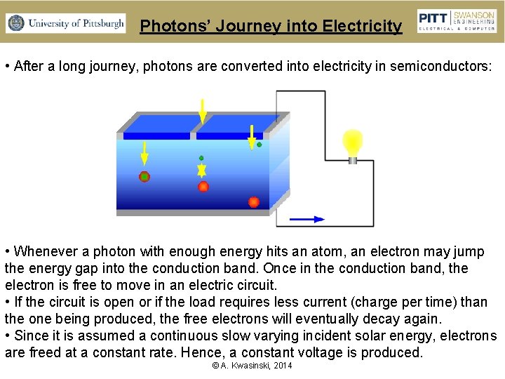
Photons’ Journey into Electricity • After a long journey, photons are converted into electricity in semiconductors: • Whenever a photon with enough energy hits an atom, an electron may jump the energy gap into the conduction band. Once in the conduction band, the electron is free to move in an electric circuit. • If the circuit is open or if the load requires less current (charge per time) than the one being produced, the free electrons will eventually decay again. • Since it is assumed a continuous slow varying incident solar energy, electrons are freed at a constant rate. Hence, a constant voltage is produced. © A. Kwasinski, 2014

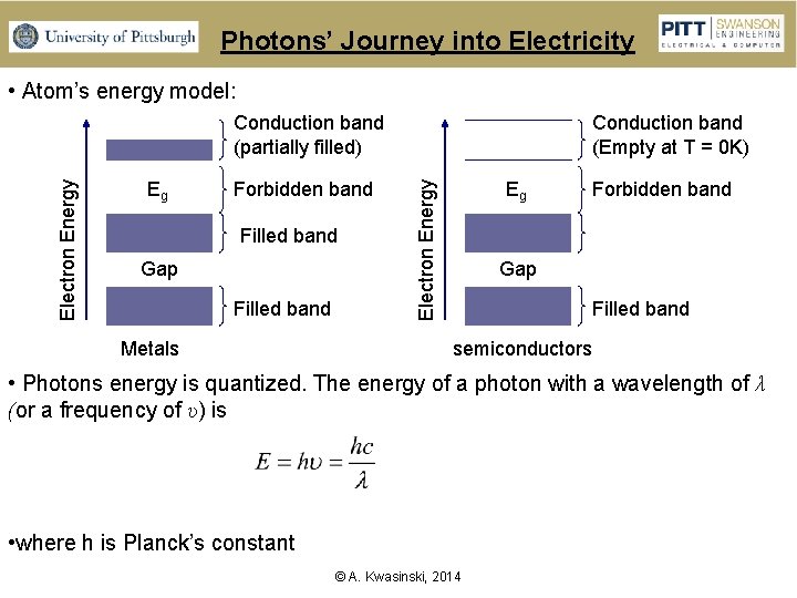
Photons’ Journey into Electricity • Atom’s energy model: Eg Forbidden band Filled band Gap Filled band Metals Conduction band (Empty at T = 0 K) Eg Electron Energy Conduction band (partially filled) Forbidden band Gap Filled band semiconductors • Photons energy is quantized. The energy of a photon with a wavelength of λ (or a frequency of υ) is • where h is Planck’s constant © A. Kwasinski, 2014

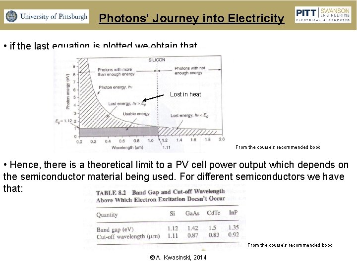
Photons’ Journey into Electricity • if the last equation is plotted we obtain that Lost in heat From the course’s recommended book • Hence, there is a theoretical limit to a PV cell power output which depends on the semiconductor material being used. For different semiconductors we have that: From the course’s recommended book © A. Kwasinski, 2014

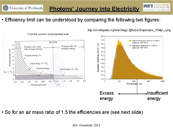
Photons’ Journey into Electricity • Efficiency limit can be understood by comparing the following two figures: http: //en. wikipedia. org/wiki/Image: Effective. Temperature_300 dpi_e. png From the course’s recommended book Excess energy • So for an air mass ratio of 1. 5 the efficiencies are (see next slide) © A. Kwasinski, 2014 Insufficient energy

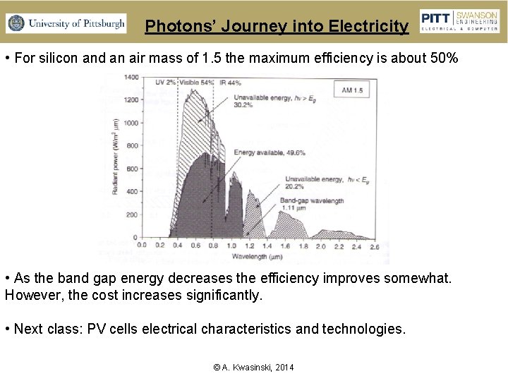
Photons’ Journey into Electricity • For silicon and an air mass of 1. 5 the maximum efficiency is about 50% • As the band gap energy decreases the efficiency improves somewhat. However, the cost increases significantly. • Next class: PV cells electrical characteristics and technologies. © A. Kwasinski, 2014

PV Cells Technologies • Characterization criterion: • Thickness: • Conventional – thick cells (200 - 500 μm) • Thin film (1 – 10 μm). Tend to be less costly than conventional (think) cells but they also tend to be less reliable and efficient. • Crystalline configuration: • Single crystal • Multicrystalline: cell formed by 1 mm to 10 cm single crystal areas. • Polycrystalline: cell formed by 1μm to 1 mm single crystal areas. • Microcrystalline: cell formed by areas of less than 1μm across. • Amorphous: No single crystal areas. • p and n region materials: • Same material: homojunction (Si) • Different material: heterojunction (Cd. S and Cu. In. Se 2) © A. Kwasinski, 2014

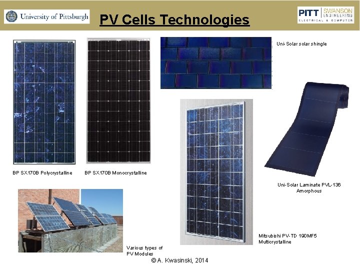
PV Cells Technologies Uni-Solar shingle BP SX 170 B Polycrystalline BP SX 170 B Monocrystalline Uni-Solar Laminate PVL-136 Amorphous Mitsubishi PV-TD 190 MF 5 Multicrystalline Various types of PV Modules © A. Kwasinski, 2014

PV Cells Technologies • Thick film fabrication techniques: • Czochraski’s (CZ): for single-crystal silicon. Costly. • Float zone process (FZ): also for single-crystal silicon. Costly • Ribbon silicon • Cast silicon: for multicrystalline cells. Less costly. • Thin film • Can be used embedded in semitransparent windows. • Techniques: • Amorphous Silicon: can achieve higher efficiencies (in the order of 42% thanks to the multijunction (different multiple layers) in which each layer absorb photons with different energy. • Gallium Arsenide (Ga. As): relatively high theoretical efficiency (29 %) which is not significantly affected by temperature. Less sensitive to radiation. Gallium makes this solution relatively expensive. • Gallium Indium Phosphide (Ga. In. P): similar to Ga. As. • Cadmium Telluride (Cd. Te): Issue: Cd is a health hazard (it is very toxic). • Copper Indium Diselenide (CIS or Cu. In. Se 2): relatively good efficiency) • Silicon Nitrade (N 4 Si 3) © A. Kwasinski, 2014

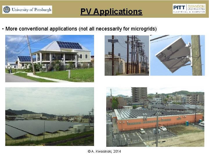
PV Applications • More conventional applications (not all necessarily for microgrids) © A. Kwasinski, 2014

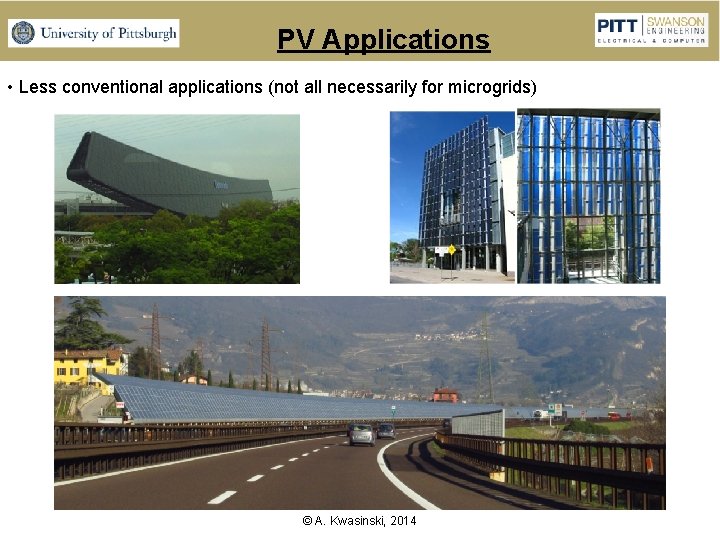
PV Applications • Less conventional applications (not all necessarily for microgrids) © A. Kwasinski, 2014

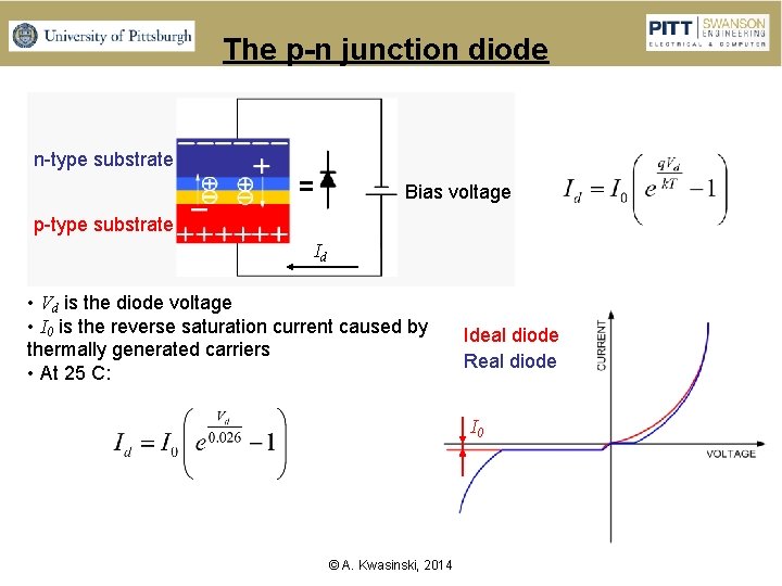
The p-n junction diode n-type substrate Bias voltage p-type substrate Id • Vd is the diode voltage • I 0 is the reverse saturation current caused by thermally generated carriers • At 25 C: Ideal diode Real diode I 0 © A. Kwasinski, 2014

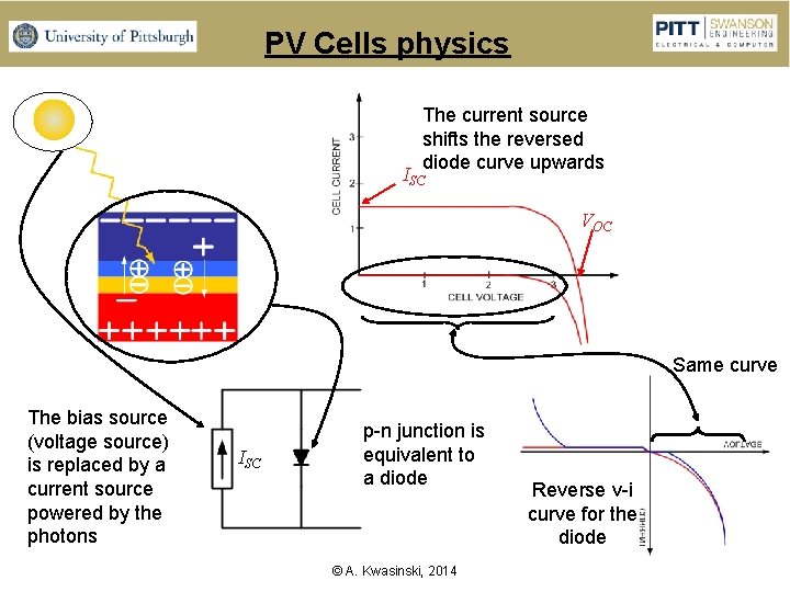
PV Cells physics The current source shifts the reversed diode curve upwards ISC VOC Same curve The bias source (voltage source) is replaced by a current source powered by the photons ISC p-n junction is equivalent to a diode © A. Kwasinski, 2014 Reverse v-i curve for the diode

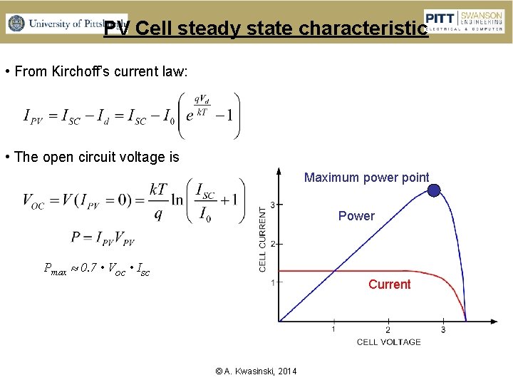
PV Cell steady state characteristic • From Kirchoff’s current law: • The open circuit voltage is Maximum power point Power Pmax 0. 7 • Voc • Isc Current © A. Kwasinski, 2014

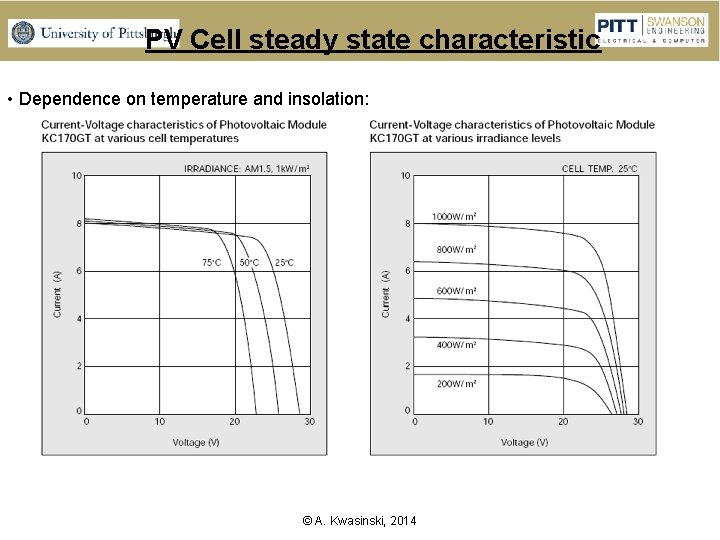
PV Cell steady state characteristic • Dependence on temperature and insolation: © A. Kwasinski, 2014

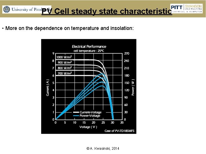
PV Cell steady state characteristic • More on the dependence on temperature and insolation: © A. Kwasinski, 2014

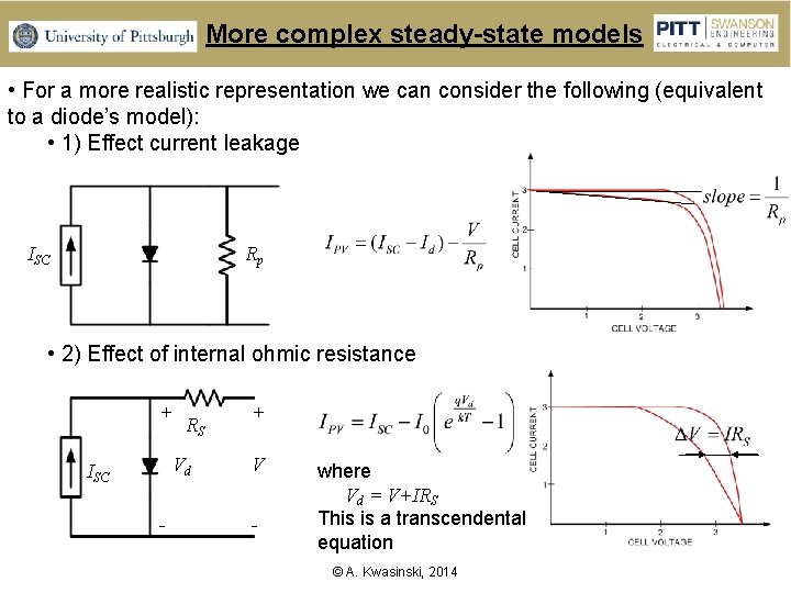
More complex steady-state models • For a more realistic representation we can consider the following (equivalent to a diode’s model): • 1) Effect current leakage ISC Rp • 2) Effect of internal ohmic resistance + RS Vd ISC - + V - where Vd = V+IRS This is a transcendental equation © A. Kwasinski, 2014

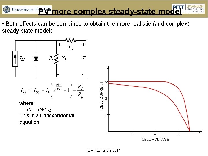
PV more complex steady-state model • Both effects can be combined to obtain the more realistic (and complex) steady state model: + ISC Rp RS Vd - + V - where Vd = V+IRS This is a transcendental equation © A. Kwasinski, 2014

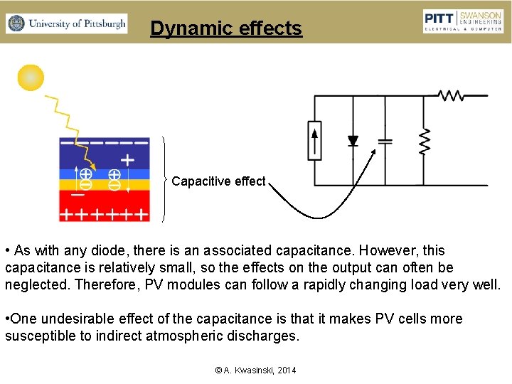
Dynamic effects Capacitive effect • As with any diode, there is an associated capacitance. However, this capacitance is relatively small, so the effects on the output can often be neglected. Therefore, PV modules can follow a rapidly changing load very well. • One undesirable effect of the capacitance is that it makes PV cells more susceptible to indirect atmospheric discharges. © A. Kwasinski, 2014

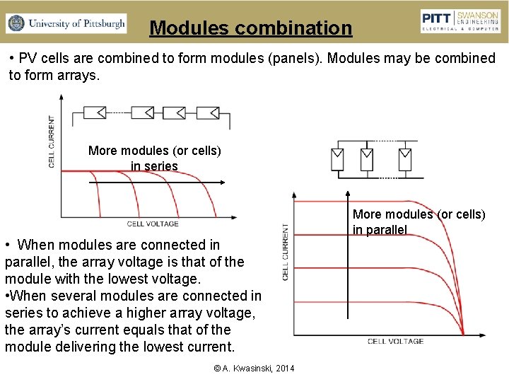
Modules combination • PV cells are combined to form modules (panels). Modules may be combined to form arrays. More modules (or cells) in series • When modules are connected in parallel, the array voltage is that of the module with the lowest voltage. • When several modules are connected in series to achieve a higher array voltage, the array’s current equals that of the module delivering the lowest current. © A. Kwasinski, 2014 More modules (or cells) in parallel

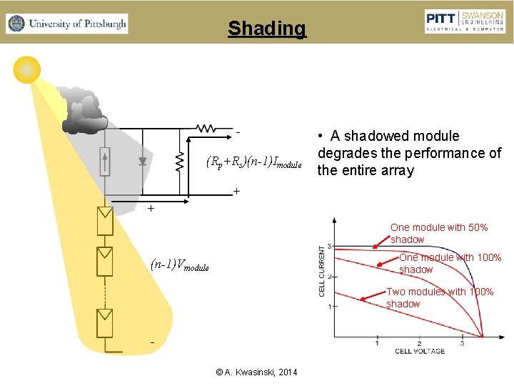
Shading (Rp+Rs)(n-1)Imodule • A shadowed module degrades the performance of the entire array + + One module with 50% shadow One module with 100% shadow (n-1)Vmodule Two modules with 100% shadow © A. Kwasinski, 2014

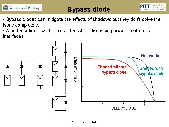
Bypass diode • Bypass diodes can mitigate the effects of shadows but they don’t solve the issue completely. • A better solution will be presented when discussing power electronics interfaces. No shade Shaded without bypass diode © A. Kwasinski, 2014 Shaded with bypass diode

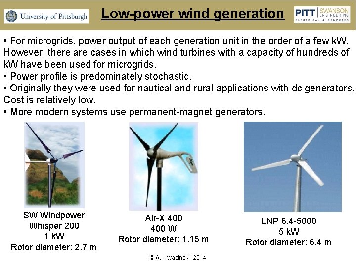
Low-power wind generation • For microgrids, power output of each generation unit in the order of a few k. W. However, there are cases in which wind turbines with a capacity of hundreds of k. W have been used for microgrids. • Power profile is predominately stochastic. • Originally they were used for nautical and rural applications with dc generators. Cost is relatively low. • More modern systems use permanent-magnet generators. SW Windpower Whisper 200 1 k. W Rotor diameter: 2. 7 m Air-X 400 W Rotor diameter: 1. 15 m © A. Kwasinski, 2014 LNP 6. 4 -5000 5 k. W Rotor diameter: 6. 4 m

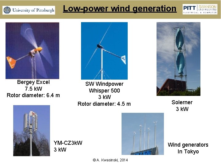
Low-power wind generation Bergey Excel 7. 5 k. W Rotor diameter: 6. 4 m SW Windpower Whisper 500 3 k. W Rotor diameter: 4. 5 m YM-CZ 3 k. W 3 k. W Solerner 3 k. W Wind generators In Tokyo © A. Kwasinski, 2014

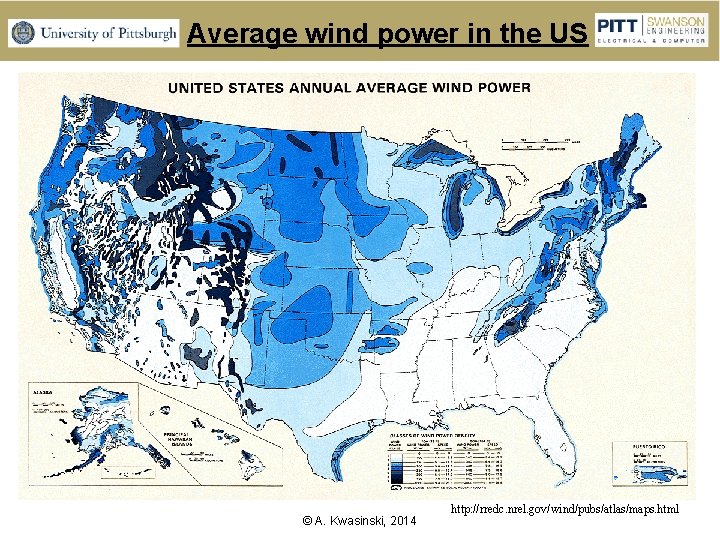
Average wind power in the US © A. Kwasinski, 2014 http: //rredc. nrel. gov/wind/pubs/atlas/maps. html

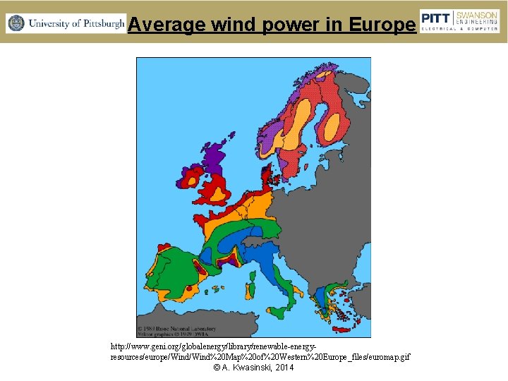
Average wind power in Europe http: //www. geni. org/globalenergy/library/renewable-energyresources/europe/Wind%20 Map%20 of%20 Western%20 Europe_files/euromap. gif © A. Kwasinski, 2014

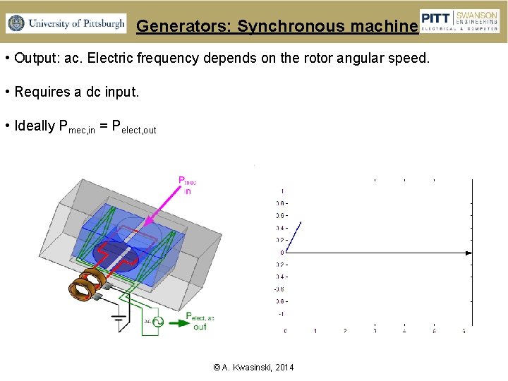
Generators: Synchronous machine • Output: ac. Electric frequency depends on the rotor angular speed. • Requires a dc input. • Ideally Pmec, in = Pelect, out © A. Kwasinski, 2014

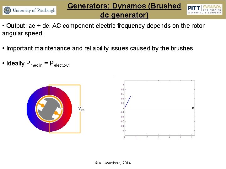
Generators: Dynamos (Brushed dc generator) • Output: ac + dc. AC component electric frequency depends on the rotor angular speed. • Important maintenance and reliability issues caused by the brushes • Ideally Pmec, in = Pelect, out © A. Kwasinski, 2014

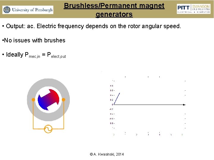
Brushless/Permanent magnet generators • Output: ac. Electric frequency depends on the rotor angular speed. • No issues with brushes • Ideally Pmec, in = Pelect, out © A. Kwasinski, 2014

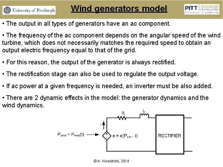
Wind generators model • The output in all types of generators have an ac component. • The frequency of the ac component depends on the angular speed of the wind turbine, which does not necessarily matches the required speed to obtain an output electric frequency equal to that of the grid. • For this reason, the output of the generator is always rectified. • The rectification stage can also be used to regulate the output voltage. • If ac power at a given frequency is needed, an inverter must be also added. • There are 2 dynamic effects in the model: the generator dynamics and the wind dynamics. © A. Kwasinski, 2014

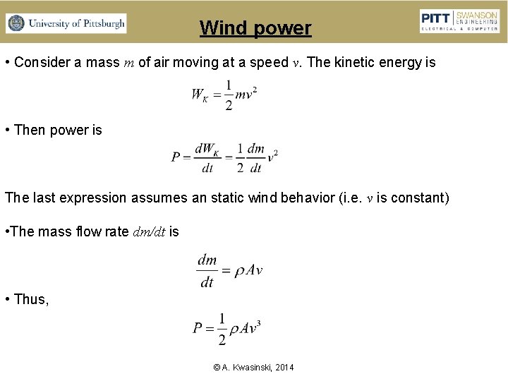
Wind power • Consider a mass m of air moving at a speed v. The kinetic energy is • Then power is The last expression assumes an static wind behavior (i. e. v is constant) • The mass flow rate dm/dt is • Thus, © A. Kwasinski, 2014

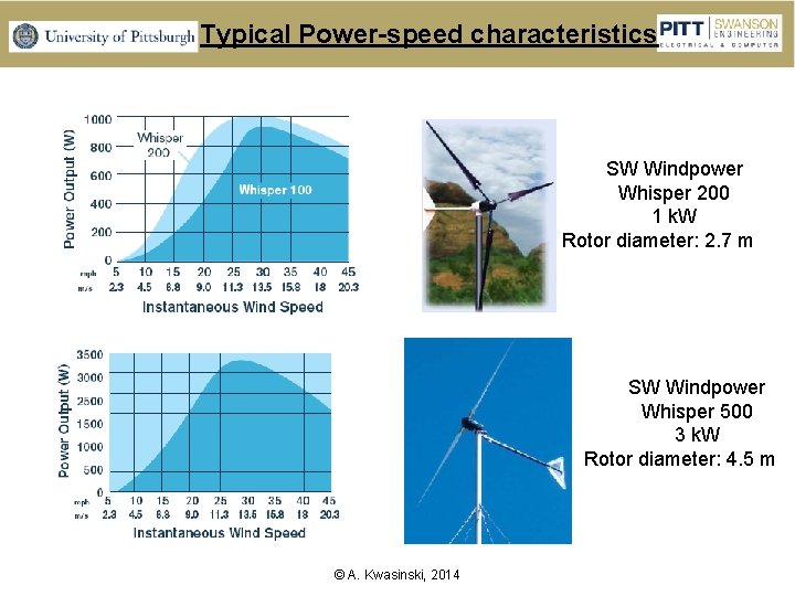
Typical Power-speed characteristics SW Windpower Whisper 200 1 k. W Rotor diameter: 2. 7 m SW Windpower Whisper 500 3 k. W Rotor diameter: 4. 5 m © A. Kwasinski, 2014

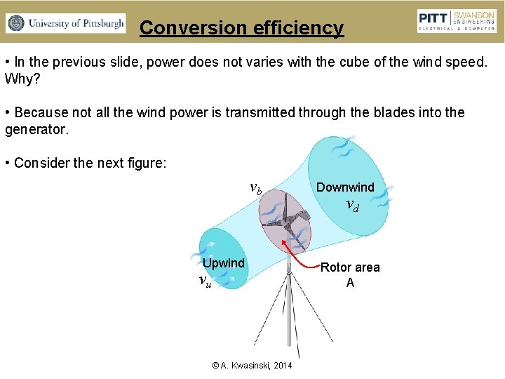
Conversion efficiency • In the previous slide, power does not varies with the cube of the wind speed. Why? • Because not all the wind power is transmitted through the blades into the generator. • Consider the next figure: vb Upwind vu © A. Kwasinski, 2014 Downwind vd Rotor area A

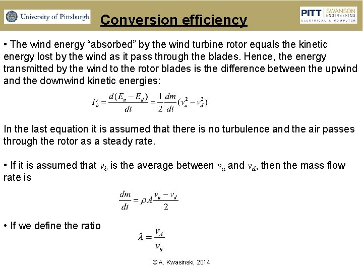
Conversion efficiency • The wind energy “absorbed” by the wind turbine rotor equals the kinetic energy lost by the wind as it pass through the blades. Hence, the energy transmitted by the wind to the rotor blades is the difference between the upwind and the downwind kinetic energies: In the last equation it is assumed that there is no turbulence and the air passes through the rotor as a steady rate. • If it is assumed that vb is the average between vu and vd, then the mass flow rate is • If we define the ratio © A. Kwasinski, 2014

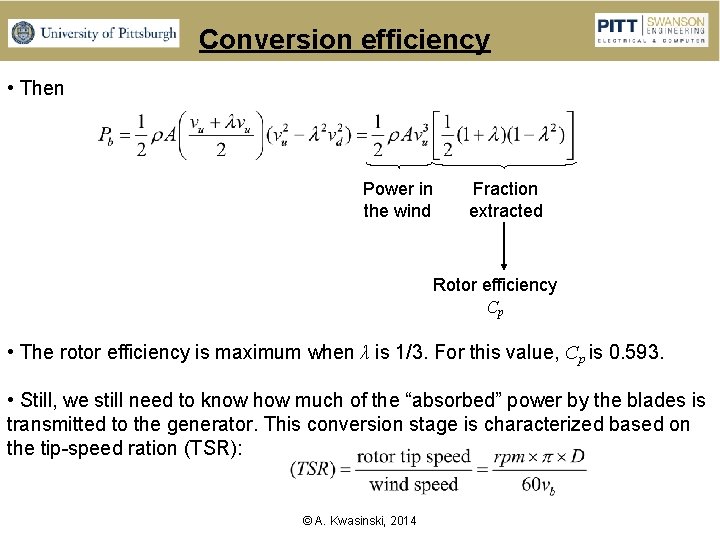
Conversion efficiency • Then Power in the wind Fraction extracted Rotor efficiency Cp • The rotor efficiency is maximum when λ is 1/3. For this value, Cp is 0. 593. • Still, we still need to know how much of the “absorbed” power by the blades is transmitted to the generator. This conversion stage is characterized based on the tip-speed ration (TSR): © A. Kwasinski, 2014

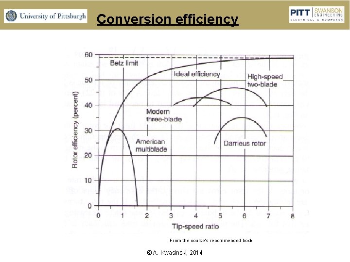
Conversion efficiency From the course’s recommended book © A. Kwasinski, 2014

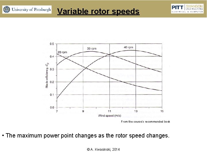
Variable rotor speeds From the course’s recommended book • The maximum power point changes as the rotor speed changes. © A. Kwasinski, 2014

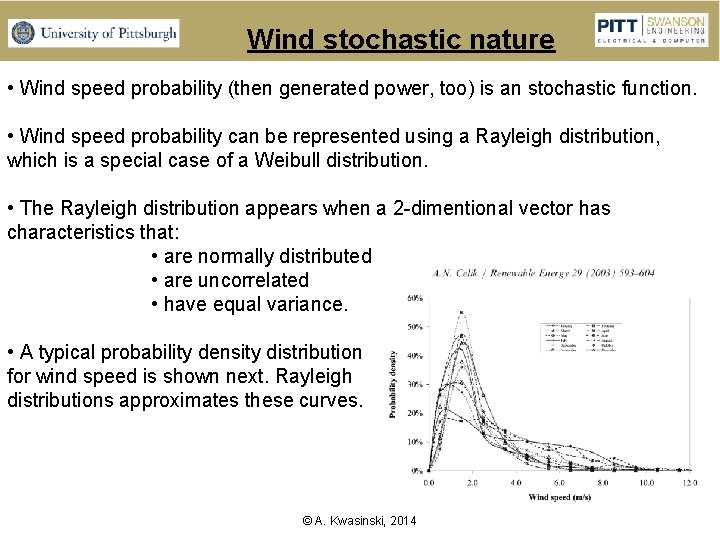
Wind stochastic nature • Wind speed probability (then generated power, too) is an stochastic function. • Wind speed probability can be represented using a Rayleigh distribution, which is a special case of a Weibull distribution. • The Rayleigh distribution appears when a 2 -dimentional vector has characteristics that: • are normally distributed • are uncorrelated • have equal variance. • A typical probability density distribution for wind speed is shown next. Rayleigh distributions approximates these curves. © A. Kwasinski, 2014

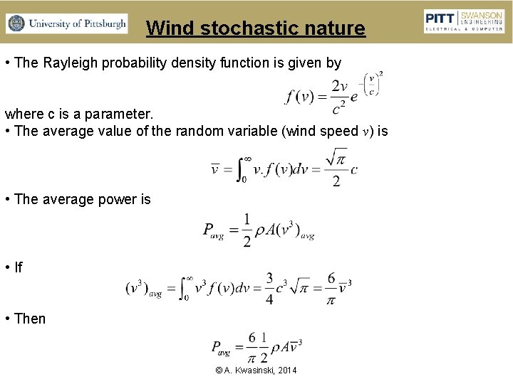
Wind stochastic nature • The Rayleigh probability density function is given by where c is a parameter. • The average value of the random variable (wind speed v) is • The average power is • If • Then © A. Kwasinski, 2014