ECE 250 Data Structures and Algorithms Laplace Transform

ECE 250 Data Structures and Algorithms Laplace Transform Douglas Wilhelm Harder Department of Electrical and Computer Engineering University of Waterloo Copyright © 2008 by Douglas Wilhelm Harder. All rights reserved.

Laplace Transform Outline • In this talk, we will: – Definition of the Laplace transform – A few simple transforms – Rules – Demonstrations

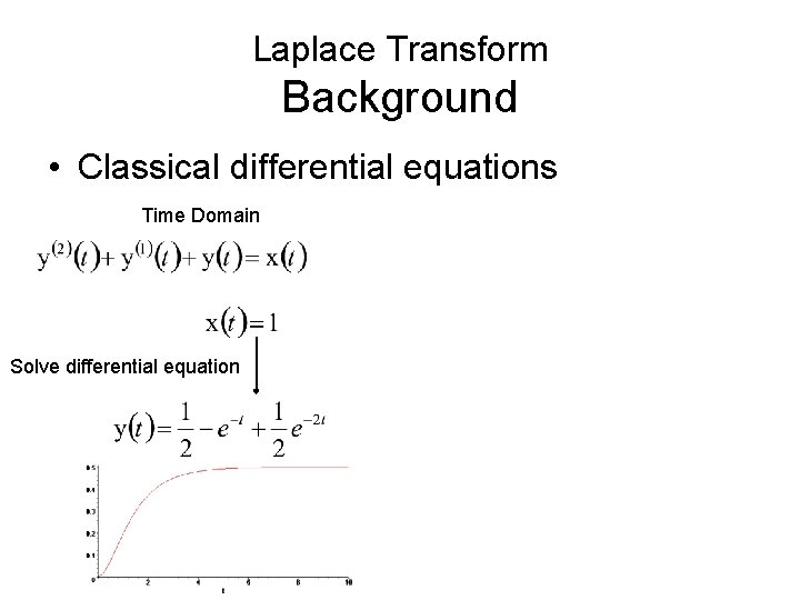
Laplace Transform Background • Classical differential equations Time Domain Solve differential equation

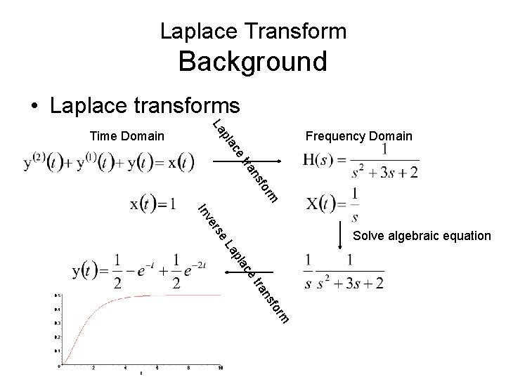
Laplace Transform Background • Laplace transforms c pla La Time Domain Frequency Domain m for ns ra et er Inv se Solve algebraic equation La pla ce m for ns tra

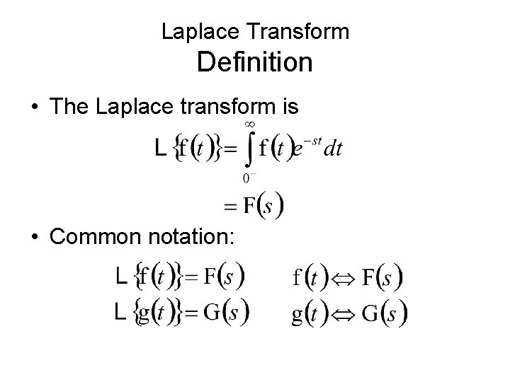
Laplace Transform Definition • The Laplace transform is • Common notation:

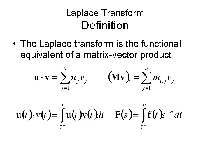
Laplace Transform Definition • The Laplace transform is the functional equivalent of a matrix-vector product

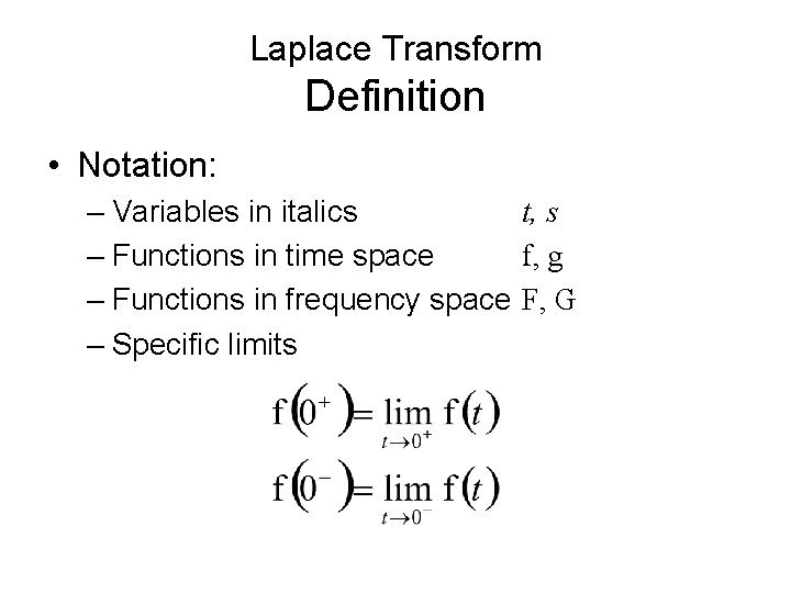
Laplace Transform Definition • Notation: – Variables in italics t, s – Functions in time space f, g – Functions in frequency space F, G – Specific limits

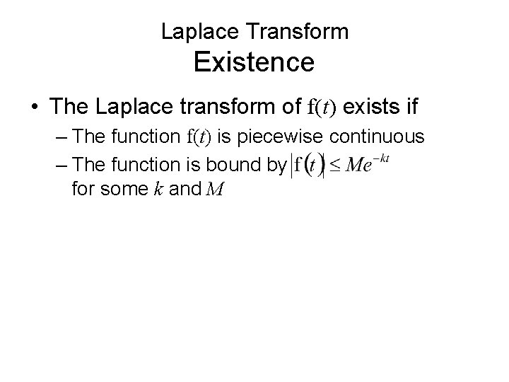
Laplace Transform Existence • The Laplace transform of f(t) exists if – The function f(t) is piecewise continuous – The function is bound by for some k and M

Laplace Transform Example Transforms • We will look at the Laplace transforms of: – The impulse function d(t) – The unit step function u(t) – The ramp function t and monomials tn – Polynomials, Taylor series, and et – Sine and cosine

Laplace Transform Example Transforms • While deriving these, we will examine certain properties: – Linearity – Damping – Time scaling – Time differentiation – Frequency differentiation

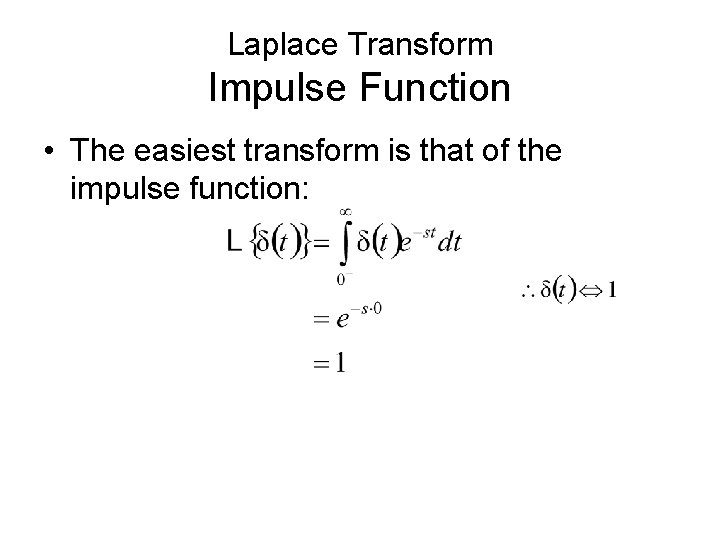
Laplace Transform Impulse Function • The easiest transform is that of the impulse function:

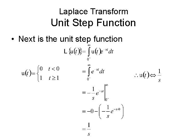
Laplace Transform Unit Step Function • Next is the unit step function

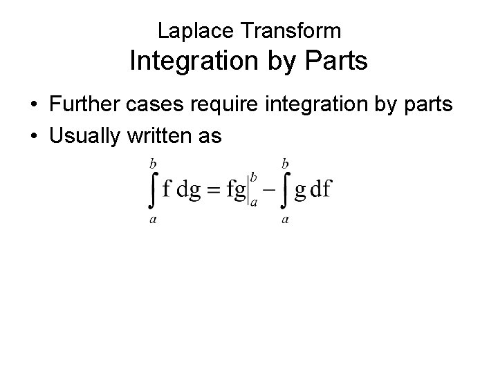
Laplace Transform Integration by Parts • Further cases require integration by parts • Usually written as

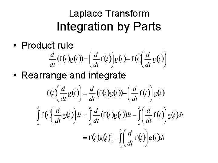
Laplace Transform Integration by Parts • Product rule • Rearrange and integrate

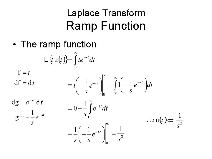
Laplace Transform Ramp Function • The ramp function

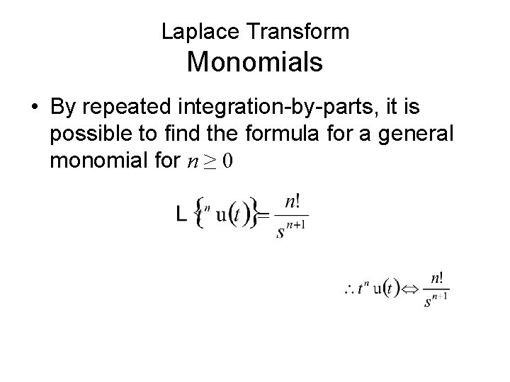
Laplace Transform Monomials • By repeated integration-by-parts, it is possible to find the formula for a general monomial for n ≥ 0

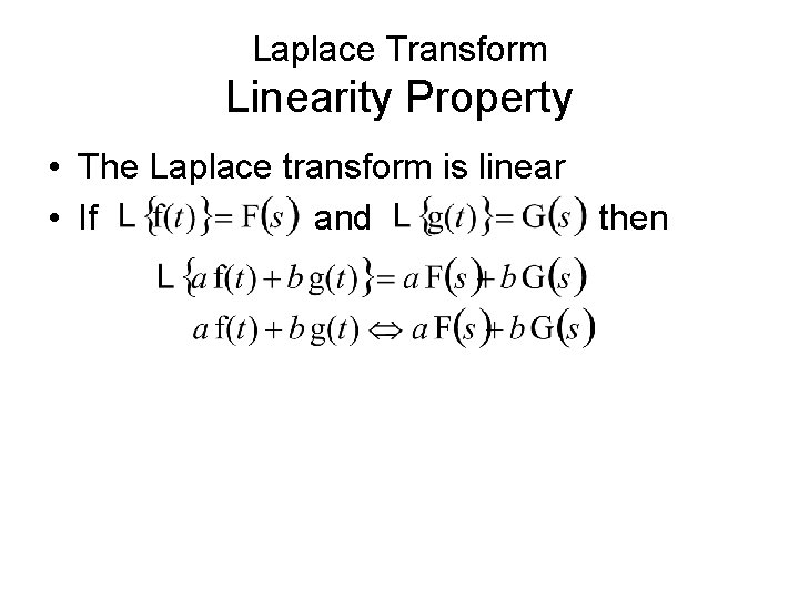
Laplace Transform Linearity Property • The Laplace transform is linear • If and then

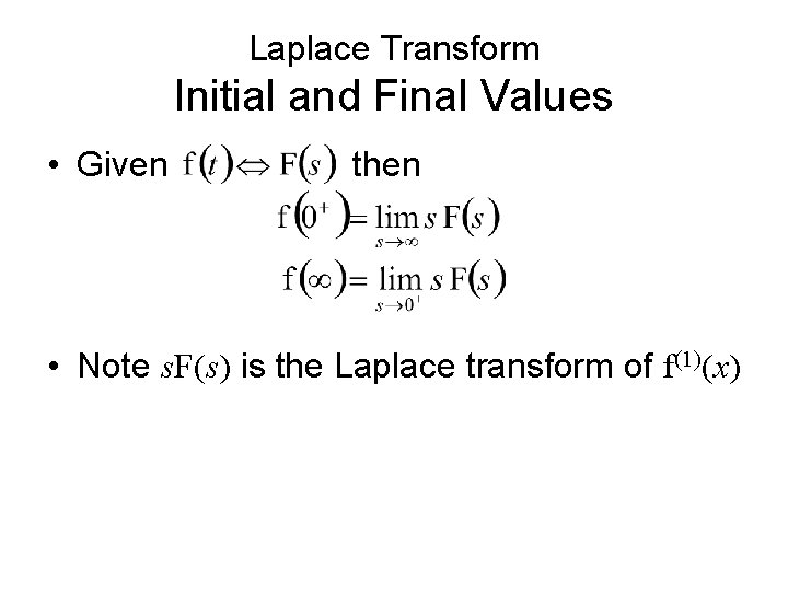
Laplace Transform Initial and Final Values • Given then • Note s. F(s) is the Laplace transform of f(1)(x)

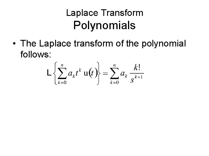
Laplace Transform Polynomials • The Laplace transform of the polynomial follows:

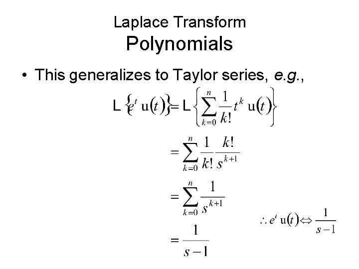
Laplace Transform Polynomials • This generalizes to Taylor series, e. g. ,

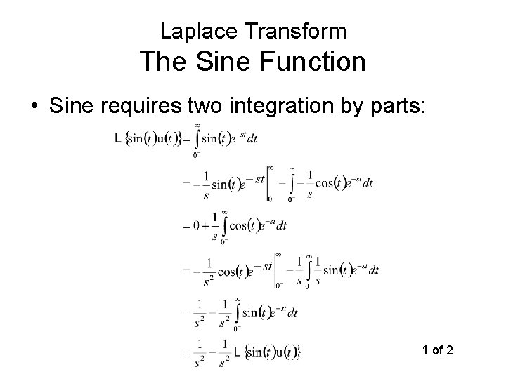
Laplace Transform The Sine Function • Sine requires two integration by parts: 1 of 2

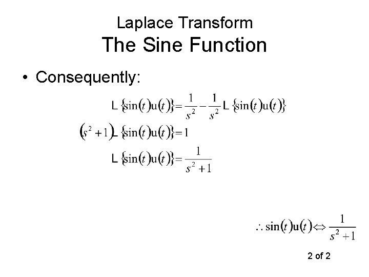
Laplace Transform The Sine Function • Consequently: 2 of 2

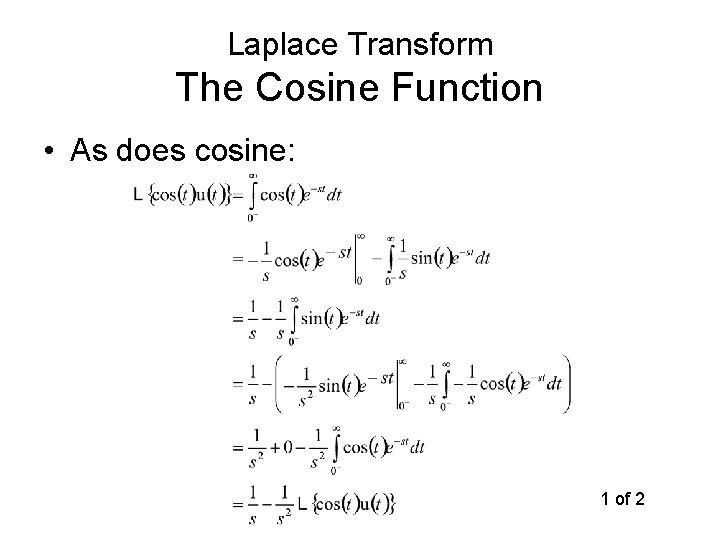
Laplace Transform The Cosine Function • As does cosine: 1 of 2

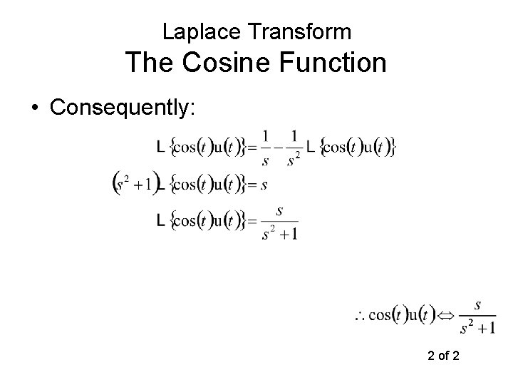
Laplace Transform The Cosine Function • Consequently: 2 of 2

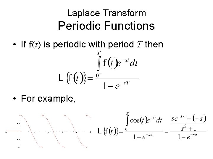
Laplace Transform Periodic Functions • If f(t) is periodic with period T then • For example,

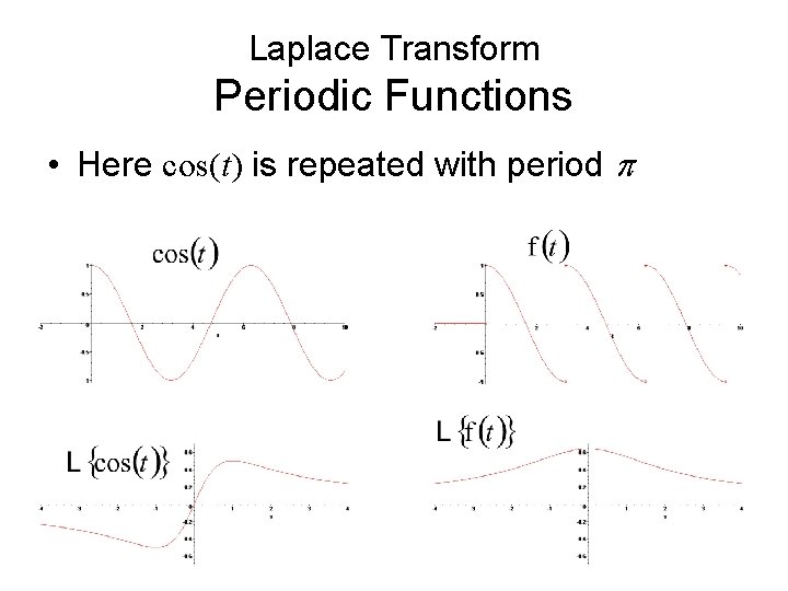
Laplace Transform Periodic Functions • Here cos(t) is repeated with period p

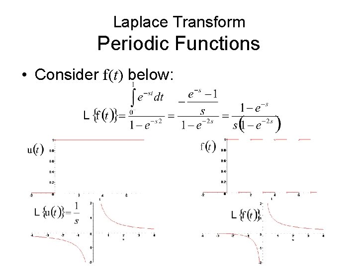
Laplace Transform Periodic Functions • Consider f(t) below:

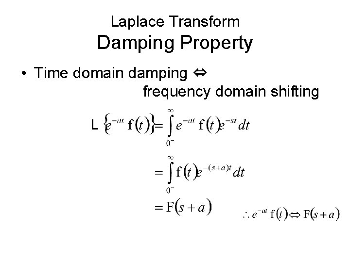
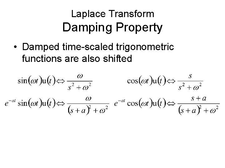
Laplace Transform Damping Property • Time domain damping ⇔ frequency domain shifting

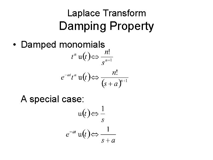
Laplace Transform Damping Property • Damped monomials A special case:

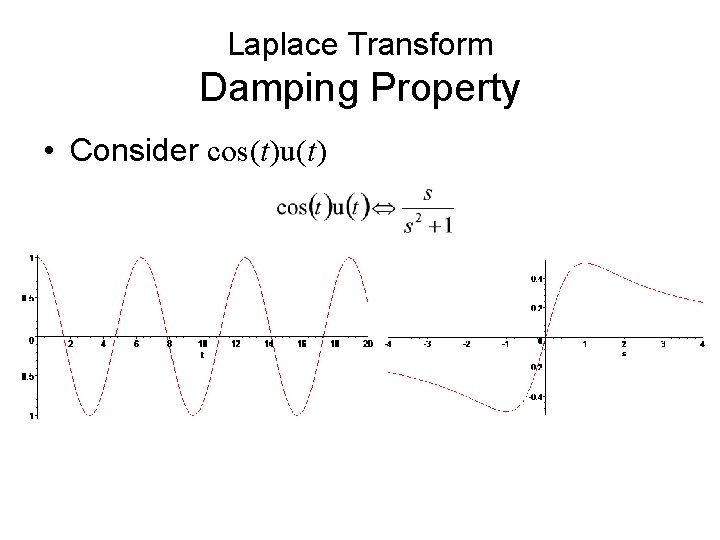
Laplace Transform Damping Property • Consider cos(t)u(t)

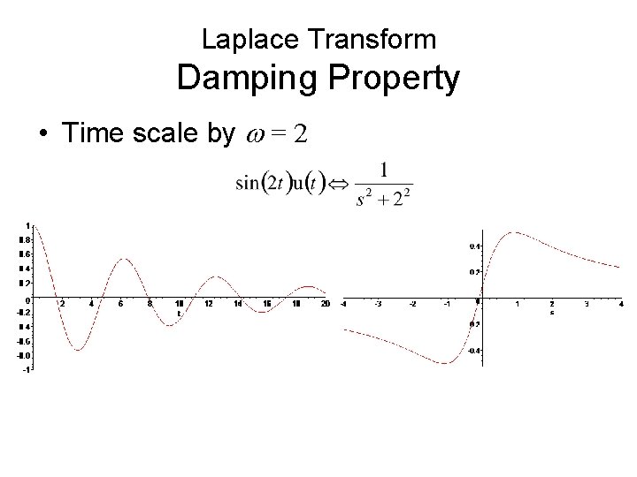
Laplace Transform Damping Property • Time scale by w = 2

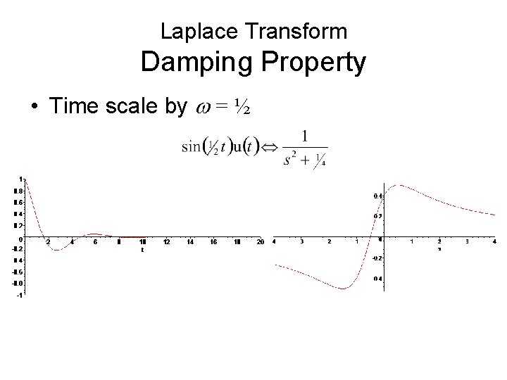
Laplace Transform Damping Property • Time scale by w = ½

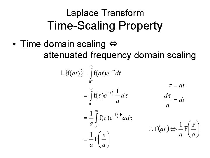
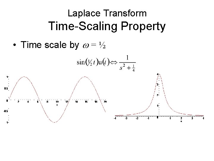
Laplace Transform Time-Scaling Property • Time domain scaling ⇔ attenuated frequency domain scaling

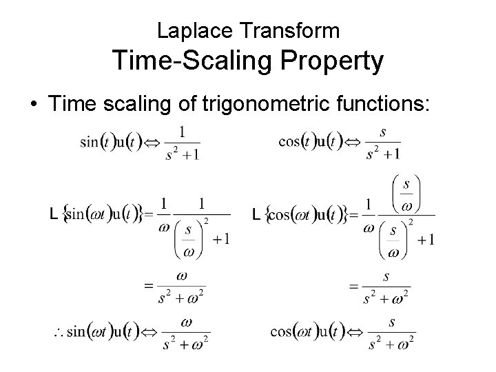
Laplace Transform Time-Scaling Property • Time scaling of trigonometric functions:

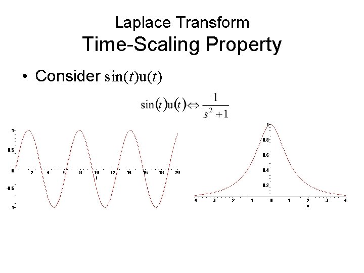
Laplace Transform Time-Scaling Property • Consider sin(t)u(t)

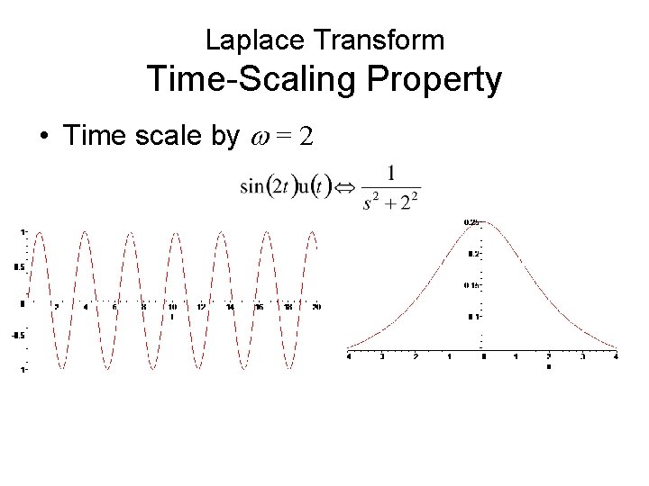
Laplace Transform Time-Scaling Property • Time scale by w = 2

Laplace Transform Time-Scaling Property • Time scale by w = ½

Laplace Transform Damping Property • Damped time-scaled trigonometric functions are also shifted

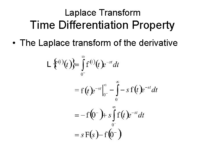
Laplace Transform Time Differentiation Property • The Laplace transform of the derivative

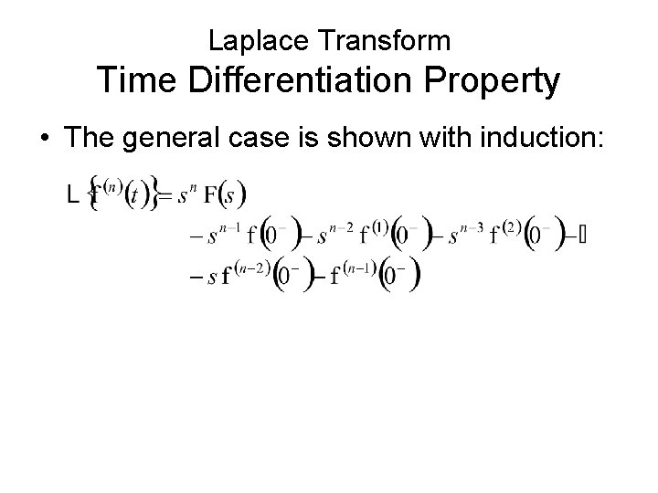
Laplace Transform Time Differentiation Property • The general case is shown with induction:

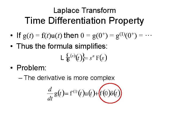
Laplace Transform Time Differentiation Property • If g(t) = f(t)u(t) then 0 = g(0+) = g(1)(0+) = ··· • Thus the formula simplifies: • Problem: – The derivative is more complex

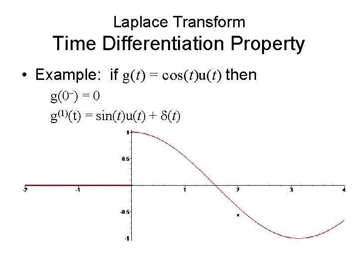
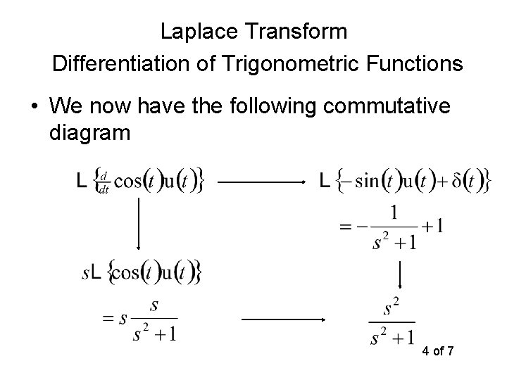
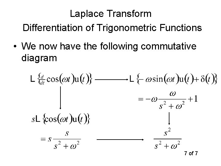
Laplace Transform Time Differentiation Property • Example: if g(t) = cos(t)u(t) then g(0–) = 0 g(1)(t) = sin(t)u(t) + d(t)

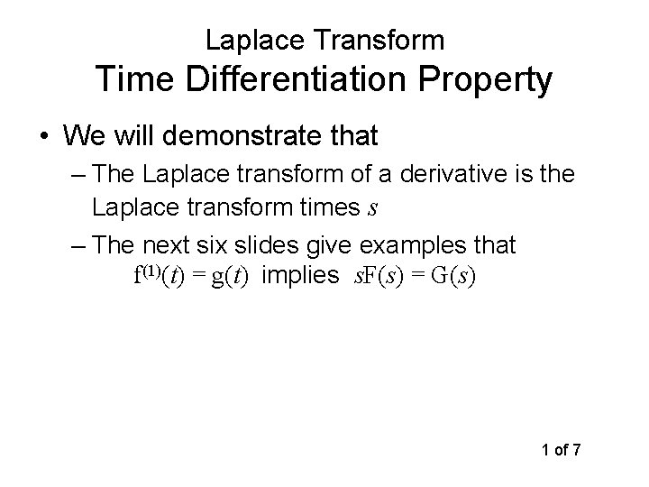
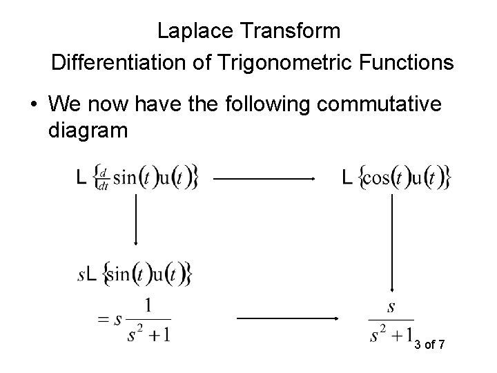
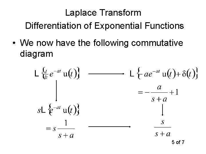
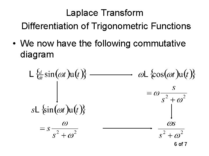
Laplace Transform Time Differentiation Property • We will demonstrate that – The Laplace transform of a derivative is the Laplace transform times s – The next six slides give examples that f(1)(t) = g(t) implies s. F(s) = G(s) 1 of 7

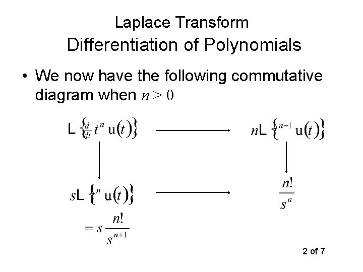
Laplace Transform Differentiation of Polynomials • We now have the following commutative diagram when n > 0 2 of 7

Laplace Transform Differentiation of Trigonometric Functions • We now have the following commutative diagram 3 of 7

Laplace Transform Differentiation of Trigonometric Functions • We now have the following commutative diagram 4 of 7

Laplace Transform Differentiation of Exponential Functions • We now have the following commutative diagram 5 of 7

Laplace Transform Differentiation of Trigonometric Functions • We now have the following commutative diagram 6 of 7

Laplace Transform Differentiation of Trigonometric Functions • We now have the following commutative diagram 7 of 7

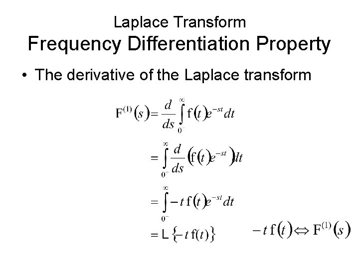
Laplace Transform Frequency Differentiation Property • The derivative of the Laplace transform

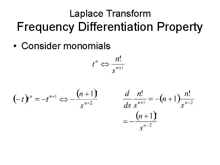
Laplace Transform Frequency Differentiation Property • Consider monomials

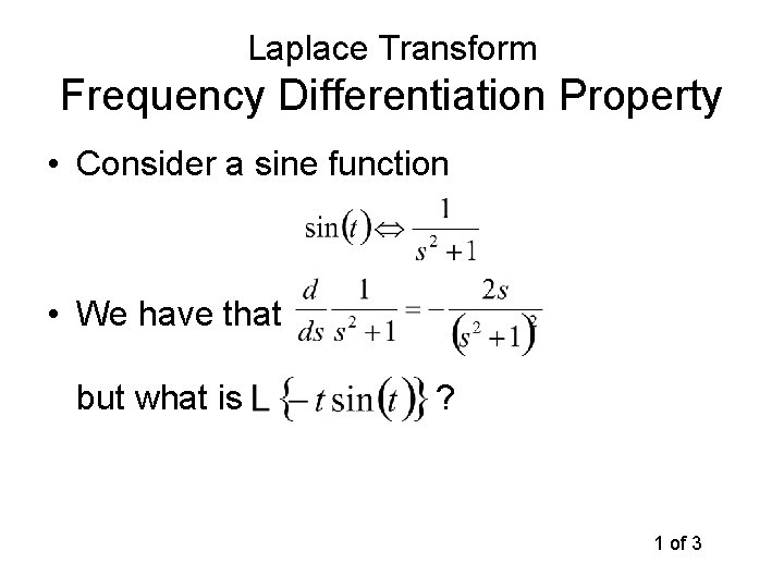
Laplace Transform Frequency Differentiation Property • Consider a sine function • We have that but what is ? 1 of 3

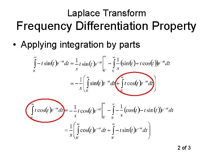
Laplace Transform Frequency Differentiation Property • Applying integration by parts 2 of 3

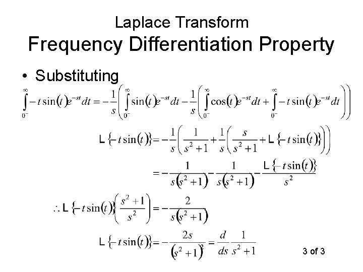
Laplace Transform Frequency Differentiation Property • Substituting 3 of 3

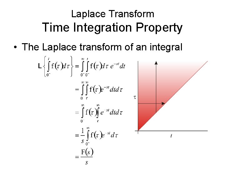
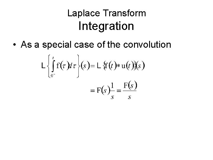
Laplace Transform Time Integration Property • The Laplace transform of an integral

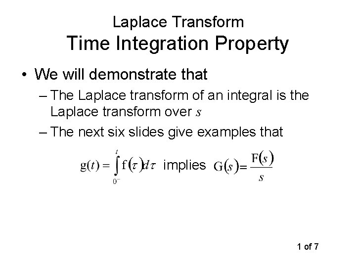
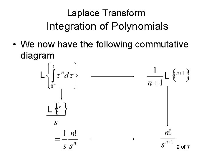
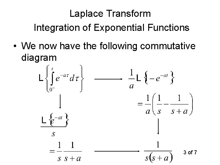
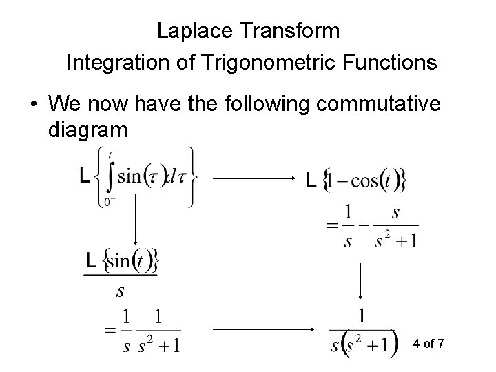
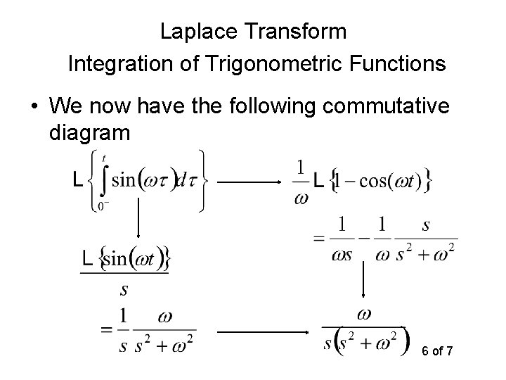
Laplace Transform Time Integration Property • We will demonstrate that – The Laplace transform of an integral is the Laplace transform over s – The next six slides give examples that implies 1 of 7

Laplace Transform Integration of Polynomials • We now have the following commutative diagram 2 of 7

Laplace Transform Integration of Exponential Functions • We now have the following commutative diagram 3 of 7

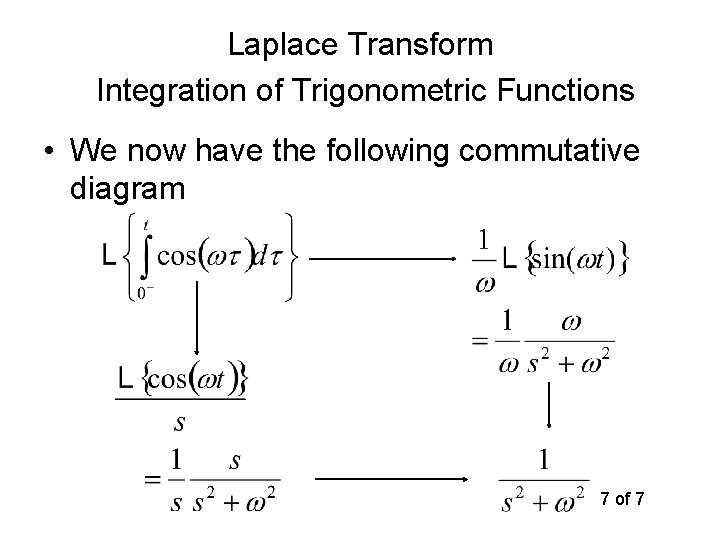
Laplace Transform Integration of Trigonometric Functions • We now have the following commutative diagram 4 of 7

Laplace Transform Integration of Trigonometric Functions • We now have the following commutative diagram 5 of 7

Laplace Transform Integration of Trigonometric Functions • We now have the following commutative diagram 6 of 7

Laplace Transform Integration of Trigonometric Functions • We now have the following commutative diagram 7 of 7

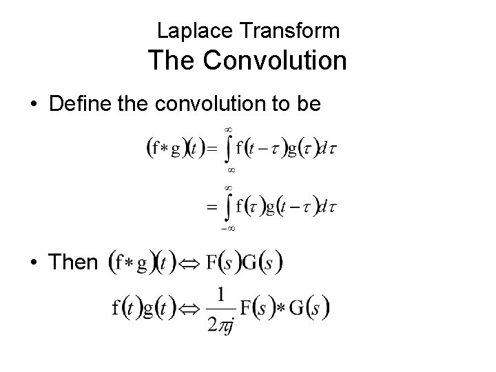
Laplace Transform The Convolution • Define the convolution to be • Then

Laplace Transform Integration • As a special case of the convolution

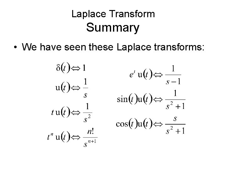
Laplace Transform Summary • We have seen these Laplace transforms:

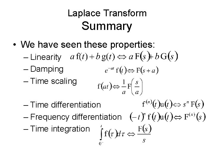
Laplace Transform Summary • We have seen these properties: – Linearity – Damping – Time scaling – Time differentiation – Frequency differentiation – Time integration

Laplace Transform Summary • In this topic: – We defined the Laplace transform – Looked at specific transforms – Derived some properties – Applied properties

Laplace Transform References • Lathi, Linear Systems and Signals, 2 nd Ed. , Oxford University Press, 2005. • Spiegel, Laplace Transforms, Mc. Graw-Hill, Inc. , 1965. • Wikipedia, http: //en. wikipedia. org/wiki/Laplace_Transform

Usage Notes • These slides are made publicly available on the web for anyone to use • If you choose to use them, or a part thereof, for a course at another institution, I ask only three things: – that you inform me that you are using the slides, – that you acknowledge my work, and – that you alert me of any mistakes which I made or changes which you make, and allow me the option of incorporating such changes (with an acknowledgment) in my set of slides Sincerely, Douglas Wilhelm Harder, MMath dwharder@alumni. uwaterloo. ca