ECE 250 Algorithms and Data Structures Linear probing

ECE 250 Algorithms and Data Structures Linear probing Douglas Wilhelm Harder, M. Math. LEL Department of Electrical and Computer Engineering University of Waterloo, Ontario, Canada ece. uwaterloo. ca dwharder@alumni. uwaterloo. ca © 2006 -2013 by Douglas Wilhelm Harder. Some rights reserved.

Linear probing 2 Outline Our first scheme for open addressing: – – Linear probing—keep looking ahead one cell at a time Examples and implementations Primary clustering Is it working looking ahead every k entries?

Linear probing 3 Linear Probing The easiest method to probe the bins of the hash table is to search forward linearly Assume we are inserting into bin k: – If bin k is empty, we occupy it – Otherwise, check bin k + 1, k + 2, and so on, until an empty bin is found • If we reach the end of the array, we start at the front (bin 0)

Linear probing 4 Linear Probing Consider a hash table with M = 16 bins Given a 3 -digit hexadecimal number: – The least-significant digit is the primary hash function (bin) – Example: for 6 B 72 A 16 , the initial bin is A and the jump size is 3

Linear probing 5 Insertion Insert these numbers into this initially empty hash table: 19 A, 207, 3 AD, 488, 5 BA, 680, 74 C, 826, 946, ACD, B 32, C 8 B, DBE, E 9 C 0 1 2 3 4 5 6 7 8 9 A B C D E F

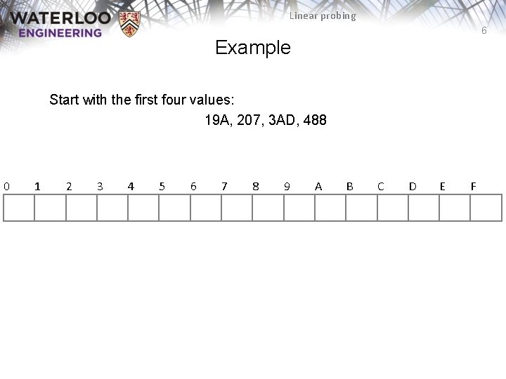
Linear probing 6 Example Start with the first four values: 19 A, 207, 3 AD, 488 0 1 2 3 4 5 6 7 8 9 A B C D E F

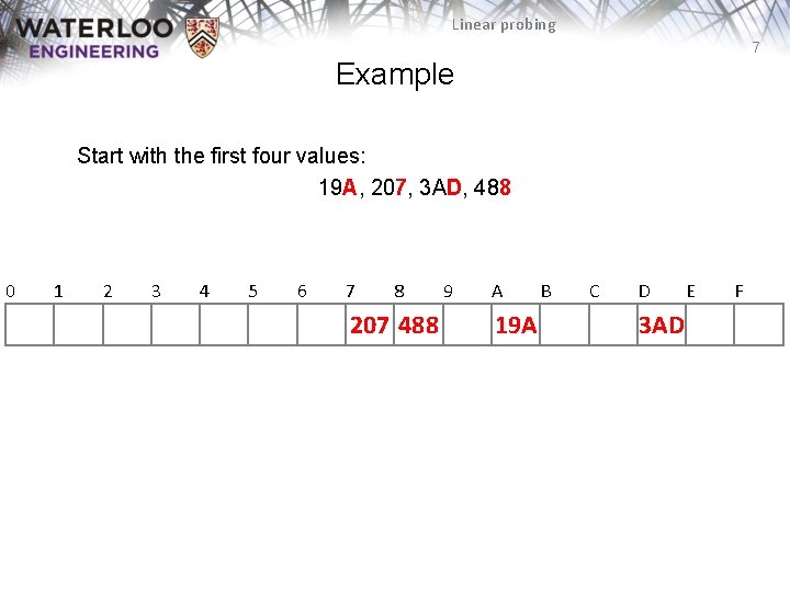
Linear probing 7 Example Start with the first four values: 19 A, 207, 3 AD, 488 0 1 2 3 4 5 6 7 8 207 488 9 A 19 A B C D 3 AD E F

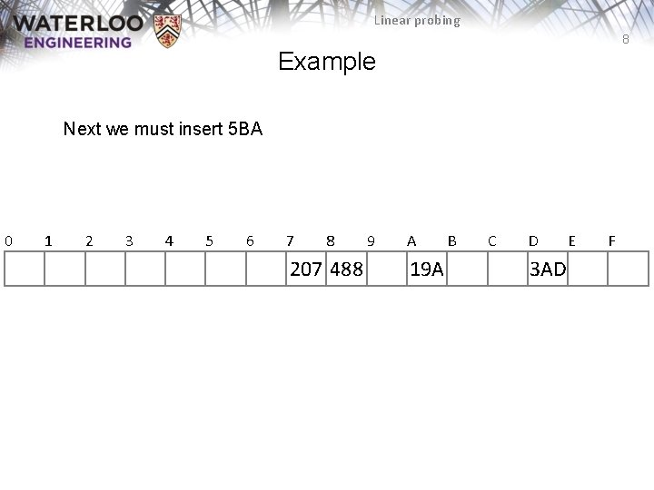
Linear probing 8 Example Next we must insert 5 BA 0 1 2 3 4 5 6 7 8 207 488 9 A 19 A B C D 3 AD E F

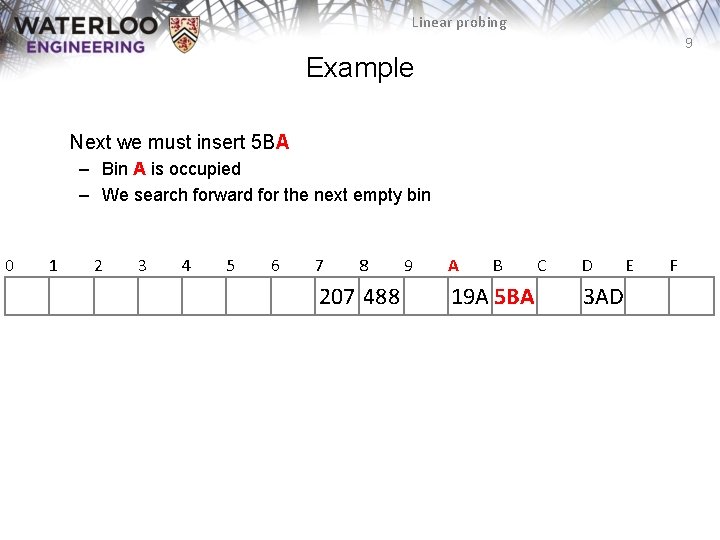
Linear probing 9 Example Next we must insert 5 BA – Bin A is occupied – We search forward for the next empty bin 0 1 2 3 4 5 6 7 8 207 488 9 A B 19 A 5 BA C D 3 AD E F

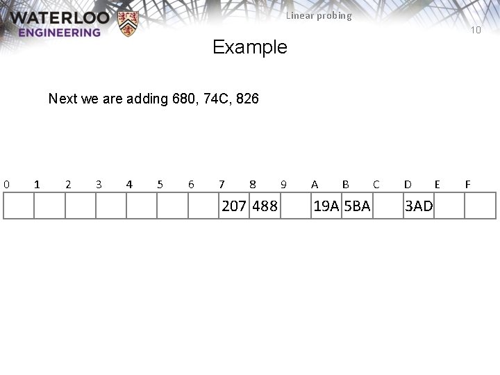
Linear probing 10 Example Next we are adding 680, 74 C, 826 0 1 2 3 4 5 6 7 8 207 488 9 A B 19 A 5 BA C D 3 AD E F

Linear probing 11 Example Next we are adding 680, 74 C, 826 – All the bins are empty—simply insert them 0 680 1 2 3 4 5 6 7 8 826 207 488 9 A B C D 19 A 5 BA 74 C 3 AD E F

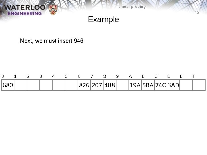
Linear probing 12 Example Next, we must insert 946 0 680 1 2 3 4 5 6 7 8 826 207 488 9 A B C D 19 A 5 BA 74 C 3 AD E F

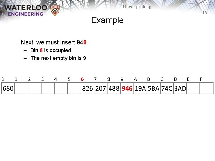
Linear probing 13 Example Next, we must insert 946 – Bin 6 is occupied – The next empty bin is 9 0 680 1 2 3 4 5 6 7 8 9 A B C D 826 207 488 946 19 A 5 BA 74 C 3 AD E F

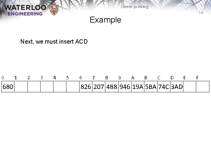
Linear probing 14 Example Next, we must insert ACD 0 680 1 2 3 4 5 6 7 8 9 A B C D 826 207 488 946 19 A 5 BA 74 C 3 AD E F

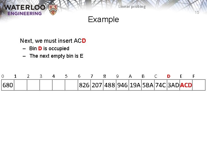
Linear probing 15 Example Next, we must insert ACD – Bin D is occupied – The next empty bin is E 0 680 1 2 3 4 5 6 7 8 9 A B C D E 826 207 488 946 19 A 5 BA 74 C 3 AD ACD F

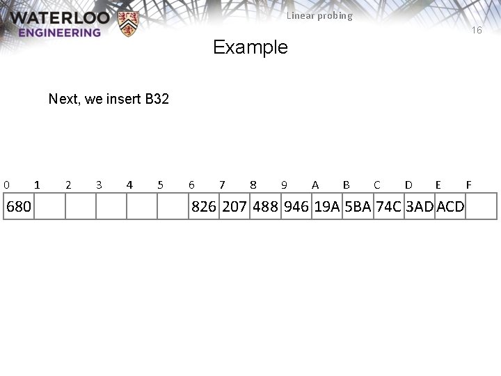
Linear probing 16 Example Next, we insert B 32 0 680 1 2 3 4 5 6 7 8 9 A B C D E 826 207 488 946 19 A 5 BA 74 C 3 AD ACD F

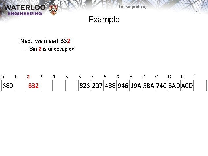
Linear probing 17 Example Next, we insert B 32 – Bin 2 is unoccupied 0 680 1 2 B 32 3 4 5 6 7 8 9 A B C D E 826 207 488 946 19 A 5 BA 74 C 3 AD ACD F

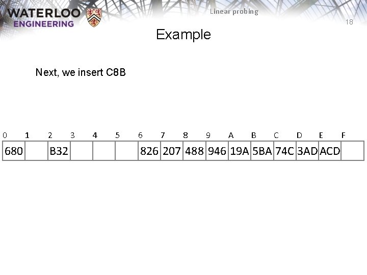
Linear probing 18 Example Next, we insert C 8 B 0 680 1 2 B 32 3 4 5 6 7 8 9 A B C D E 826 207 488 946 19 A 5 BA 74 C 3 AD ACD F

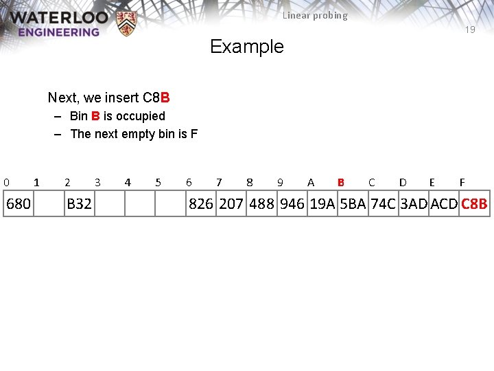
Linear probing 19 Example Next, we insert C 8 B – Bin B is occupied – The next empty bin is F 0 680 1 2 B 32 3 4 5 6 7 8 9 A B C D E F 826 207 488 946 19 A 5 BA 74 C 3 AD ACD C 8 B

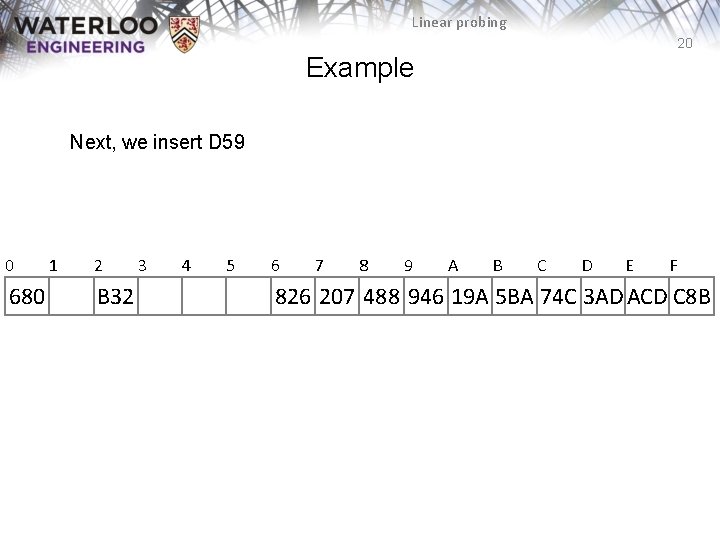
Linear probing 20 Example Next, we insert D 59 0 680 1 2 B 32 3 4 5 6 7 8 9 A B C D E F 826 207 488 946 19 A 5 BA 74 C 3 AD ACD C 8 B

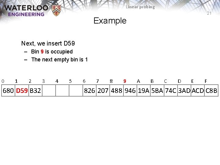
Linear probing 21 Example Next, we insert D 59 – Bin 9 is occupied – The next empty bin is 1 0 1 2 680 D 59 B 32 3 4 5 6 7 8 9 A B C D E F 826 207 488 946 19 A 5 BA 74 C 3 AD ACD C 8 B

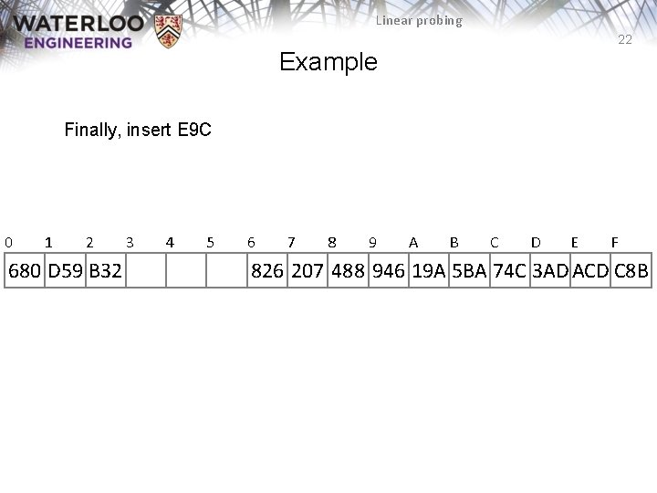
Linear probing 22 Example Finally, insert E 9 C 0 1 2 680 D 59 B 32 3 4 5 6 7 8 9 A B C D E F 826 207 488 946 19 A 5 BA 74 C 3 AD ACD C 8 B

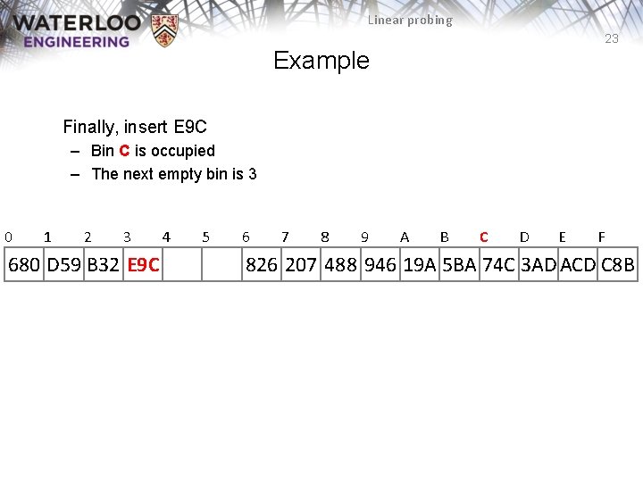
Linear probing 23 Example Finally, insert E 9 C – Bin C is occupied – The next empty bin is 3 0 1 2 3 680 D 59 B 32 E 9 C 4 5 6 7 8 9 A B C D E F 826 207 488 946 19 A 5 BA 74 C 3 AD ACD C 8 B

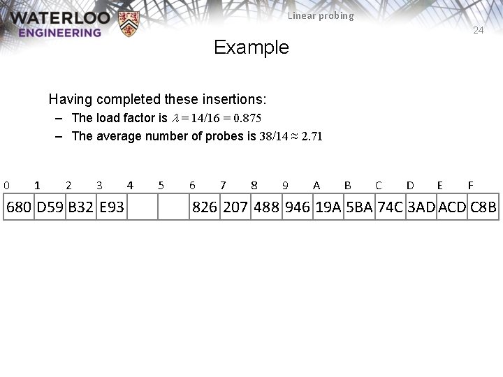
Linear probing 24 Example Having completed these insertions: – The load factor is l = 14/16 = 0. 875 – The average number of probes is 38/14 ≈ 2. 71 0 1 2 3 680 D 59 B 32 E 93 4 5 6 7 8 9 A B C D E F 826 207 488 946 19 A 5 BA 74 C 3 AD ACD C 8 B

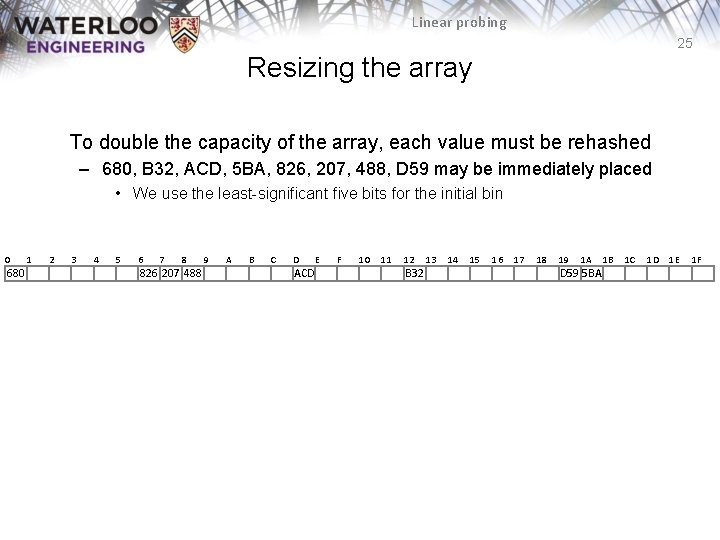
Linear probing 25 Resizing the array To double the capacity of the array, each value must be rehashed – 680, B 32, ACD, 5 BA, 826, 207, 488, D 59 may be immediately placed • We use the least-significant five bits for the initial bin 0 680 1 2 3 4 5 6 7 8 826 207 488 9 A B C D ACD E F 10 11 12 B 32 13 14 15 16 17 18 19 1 A D 59 5 BA 1 B 1 C 1 D 1 E 1 F

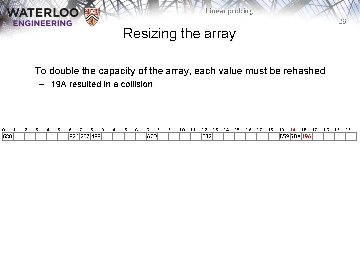
Linear probing 26 Resizing the array To double the capacity of the array, each value must be rehashed – 19 A resulted in a collision 0 680 1 2 3 4 5 6 7 8 826 207 488 9 A B C D ACD E F 10 11 12 B 32 13 14 15 16 17 18 19 1 A 1 B D 59 5 BA 19 A 1 C 1 D 1 E 1 F

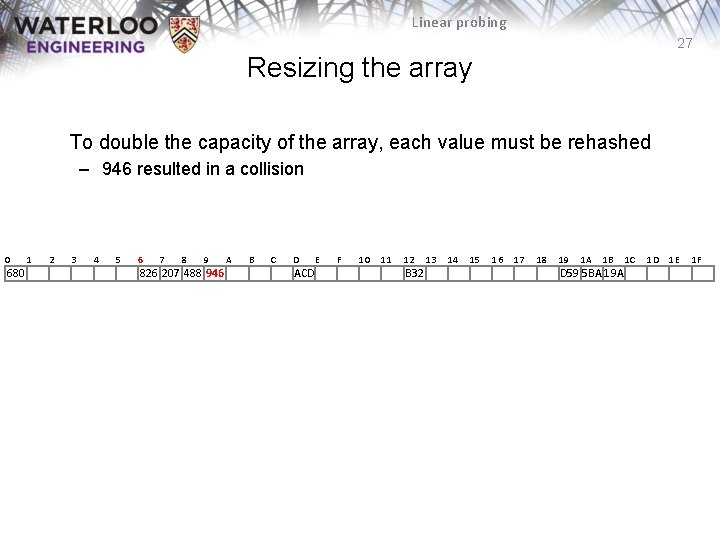
Linear probing 27 Resizing the array To double the capacity of the array, each value must be rehashed – 946 resulted in a collision 0 680 1 2 3 4 5 6 7 8 9 826 207 488 946 A B C D ACD E F 10 11 12 B 32 13 14 15 16 17 18 19 1 A 1 B D 59 5 BA 19 A 1 C 1 D 1 E 1 F

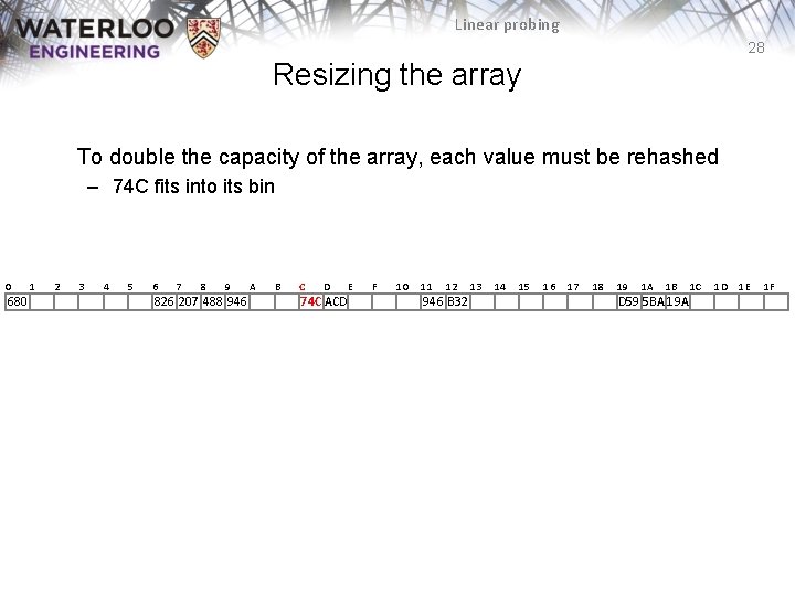
Linear probing 28 Resizing the array To double the capacity of the array, each value must be rehashed – 74 C fits into its bin 0 680 1 2 3 4 5 6 7 8 9 826 207 488 946 A B C D 74 C ACD E F 10 11 12 946 B 32 13 14 15 16 17 18 19 1 A 1 B D 59 5 BA 19 A 1 C 1 D 1 E 1 F

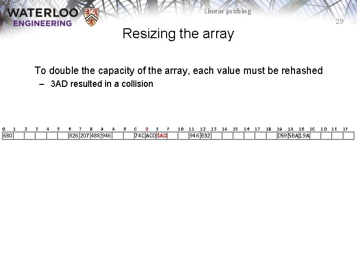
Linear probing 29 Resizing the array To double the capacity of the array, each value must be rehashed – 3 AD resulted in a collision 0 680 1 2 3 4 5 6 7 8 9 826 207 488 946 A B C D E 74 C ACD 3 AD F 10 11 12 946 B 32 13 14 15 16 17 18 19 1 A 1 B D 59 5 BA 19 A 1 C 1 D 1 E 1 F

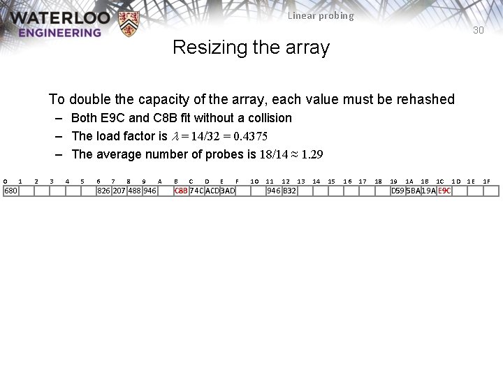
Linear probing 30 Resizing the array To double the capacity of the array, each value must be rehashed – Both E 9 C and C 8 B fit without a collision – The load factor is l = 14/32 = 0. 4375 – The average number of probes is 18/14 ≈ 1. 29 0 680 1 2 3 4 5 6 7 8 9 826 207 488 946 A B C D E C 8 B 74 C ACD 3 AD F 10 11 12 946 B 32 13 14 15 16 17 18 19 1 A 1 B 1 C D 59 5 BA 19 A E 9 C 1 D 1 E 1 F

Linear probing 31 Marking bins occupied How can we mark a bin as occupied? Pointers nullptr Positive integers -1 Floating-point numbers Na. N Objects Create a privately stored static object that does not compare to any other instances of that class Suppose we’re storing arbitrary integers? – Should we store – 1938275734 in the hopes that it will never be inserted into the hash table? – In general, magic numbers are bad—they lead to spurious errors A better solution: – Create a bit vector where the kth entry is marked true if the kth entry of the hash table is occupied

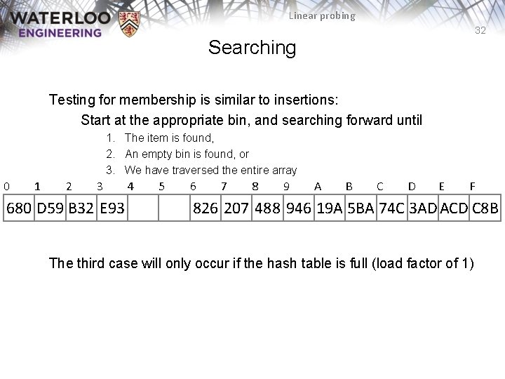
Linear probing 32 Searching Testing for membership is similar to insertions: Start at the appropriate bin, and searching forward until 1. The item is found, 2. An empty bin is found, or 3. We have traversed the entire array 0 1 2 3 680 D 59 B 32 E 93 4 5 6 7 8 9 A B C D E F 826 207 488 946 19 A 5 BA 74 C 3 AD ACD C 8 B The third case will only occur if the hash table is full (load factor of 1)

Linear probing 33 Searching for C 8 B 0 1 2 3 680 D 59 B 32 E 93 4 5 6 7 8 9 A B C D E F 826 207 488 946 19 A 5 BA 74 C 3 AD ACD C 8 B

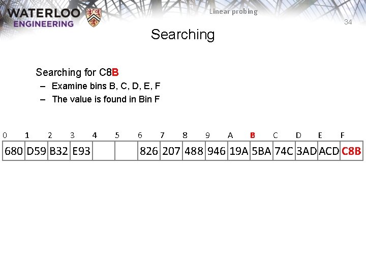
Linear probing 34 Searching for C 8 B – Examine bins B, C, D, E, F – The value is found in Bin F 0 1 2 3 680 D 59 B 32 E 93 4 5 6 7 8 9 A B C D E F 826 207 488 946 19 A 5 BA 74 C 3 AD ACD C 8 B

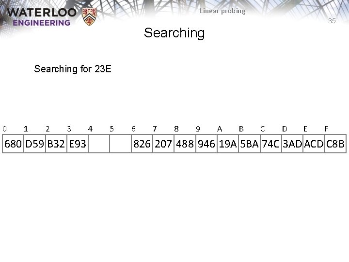
Linear probing 35 Searching for 23 E 0 1 2 3 680 D 59 B 32 E 93 4 5 6 7 8 9 A B C D E F 826 207 488 946 19 A 5 BA 74 C 3 AD ACD C 8 B

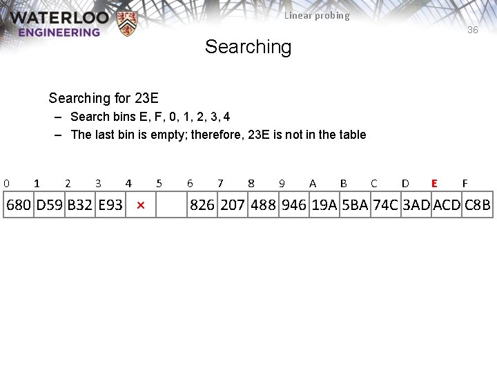
Linear probing 36 Searching for 23 E – Search bins E, F, 0, 1, 2, 3, 4 – The last bin is empty; therefore, 23 E is not in the table 0 1 2 3 4 680 D 59 B 32 E 93 × 5 6 7 8 9 A B C D E F 826 207 488 946 19 A 5 BA 74 C 3 AD ACD C 8 B

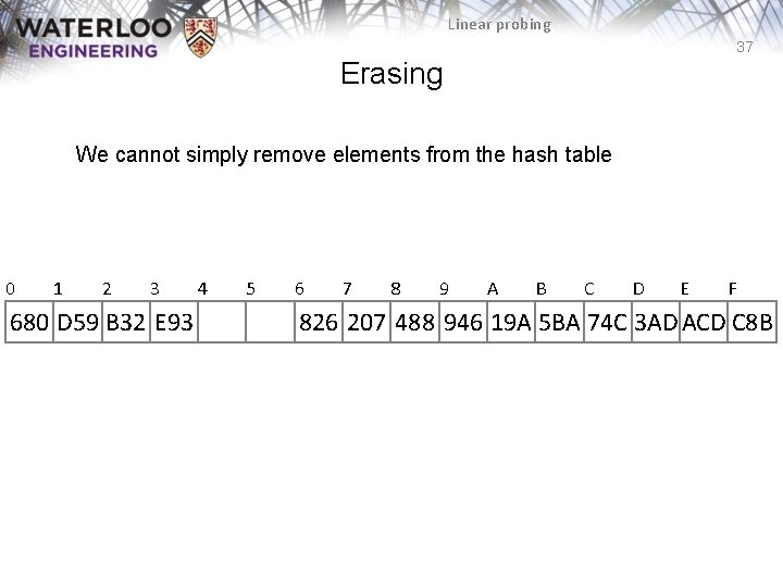
Linear probing 37 Erasing We cannot simply remove elements from the hash table 0 1 2 3 680 D 59 B 32 E 93 4 5 6 7 8 9 A B C D E F 826 207 488 946 19 A 5 BA 74 C 3 AD ACD C 8 B

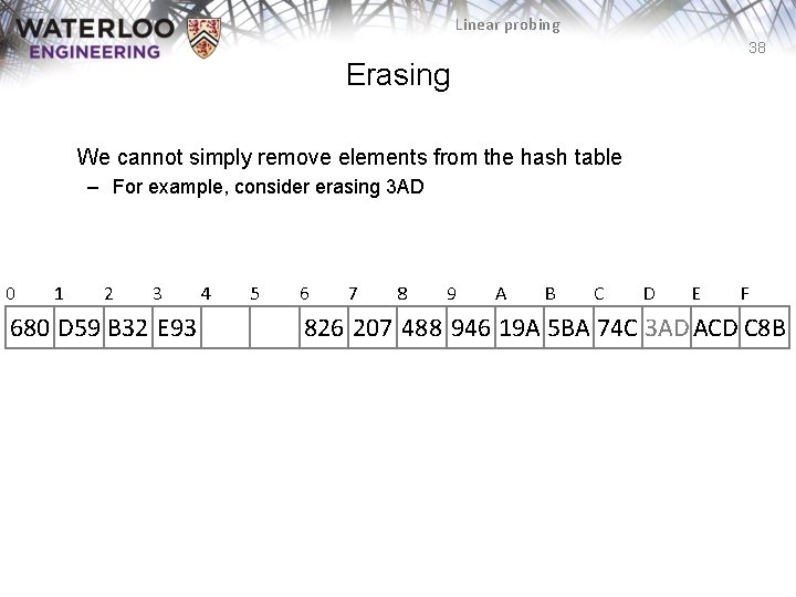
Linear probing 38 Erasing We cannot simply remove elements from the hash table – For example, consider erasing 3 AD 0 1 2 3 680 D 59 B 32 E 93 4 5 6 7 8 9 A B C D E F 826 207 488 946 19 A 5 BA 74 C 3 AD ACD C 8 B

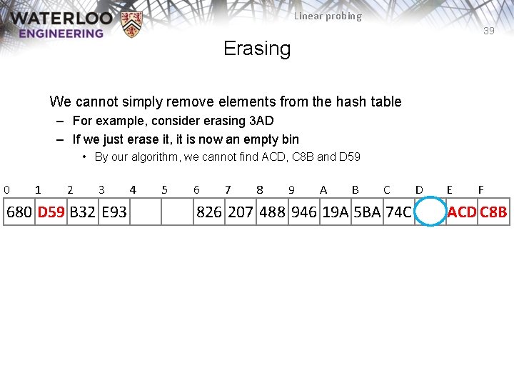
Linear probing 39 Erasing We cannot simply remove elements from the hash table – For example, consider erasing 3 AD – If we just erase it, it is now an empty bin • By our algorithm, we cannot find ACD, C 8 B and D 59 0 1 2 3 680 D 59 B 32 E 93 4 5 6 7 8 9 A B C 826 207 488 946 19 A 5 BA 74 C D E F ACD C 8 B

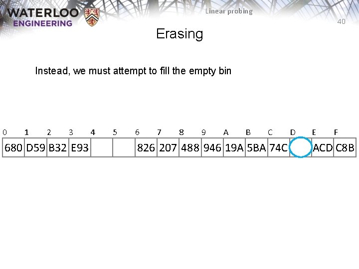
Linear probing 40 Erasing Instead, we must attempt to fill the empty bin 0 1 2 3 680 D 59 B 32 E 93 4 5 6 7 8 9 A B C 826 207 488 946 19 A 5 BA 74 C D E F ACD C 8 B

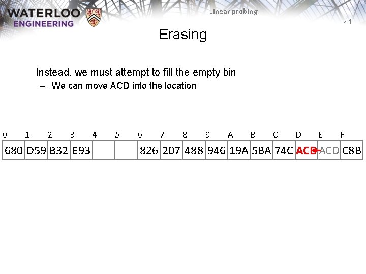
Linear probing 41 Erasing Instead, we must attempt to fill the empty bin – We can move ACD into the location 0 1 2 3 680 D 59 B 32 E 93 4 5 6 7 8 9 A B C D E F 826 207 488 946 19 A 5 BA 74 C ACD C 8 B

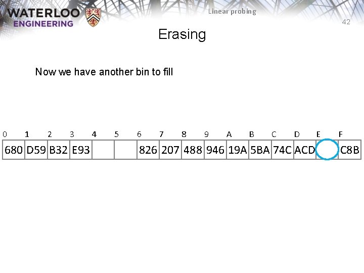
Linear probing 42 Erasing Now we have another bin to fill 0 1 2 3 680 D 59 B 32 E 93 4 5 6 7 8 9 A B C D 826 207 488 946 19 A 5 BA 74 C ACD E F C 8 B

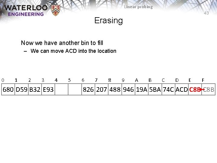
Linear probing 43 Erasing Now we have another bin to fill – We can move ACD into the location 0 1 2 3 680 D 59 B 32 E 93 4 5 6 7 8 9 A B C D E F 826 207 488 946 19 A 5 BA 74 C ACD C 8 B

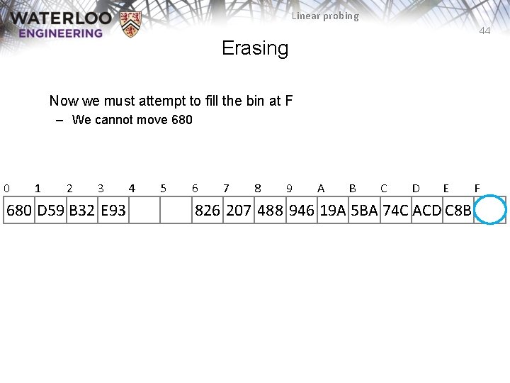
Linear probing 44 Erasing Now we must attempt to fill the bin at F – We cannot move 680 0 1 2 3 680 D 59 B 32 E 93 4 5 6 7 8 9 A B C D E 826 207 488 946 19 A 5 BA 74 C ACD C 8 B F

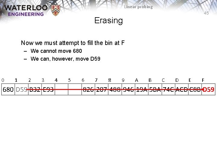
Linear probing 45 Erasing Now we must attempt to fill the bin at F – We cannot move 680 – We can, however, move D 59 0 1 2 3 680 D 59 B 32 E 93 4 5 6 7 8 9 A B C D E F 826 207 488 946 19 A 5 BA 74 C ACD C 8 B D 59

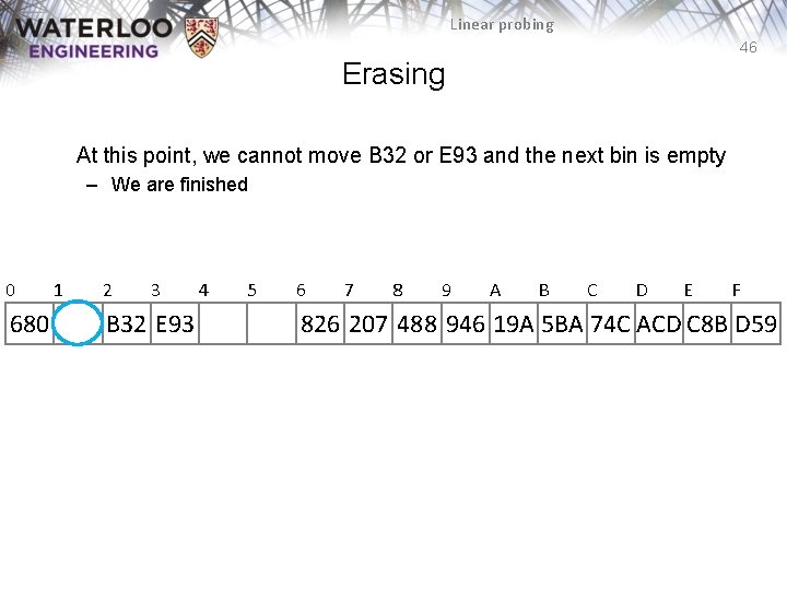
Linear probing 46 Erasing At this point, we cannot move B 32 or E 93 and the next bin is empty – We are finished 0 680 1 2 3 B 32 E 93 4 5 6 7 8 9 A B C D E F 826 207 488 946 19 A 5 BA 74 C ACD C 8 B D 59

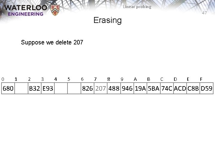
Linear probing 47 Erasing Suppose we delete 207 0 680 1 2 3 B 32 E 93 4 5 6 7 8 9 A B C D E F 826 207 488 946 19 A 5 BA 74 C ACD C 8 B D 59

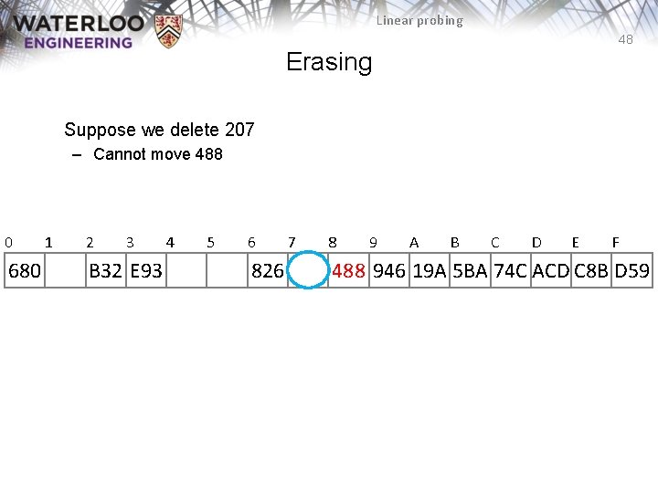
Linear probing 48 Erasing Suppose we delete 207 – Cannot move 488 0 680 1 2 3 B 32 E 93 4 5 6 826 7 8 9 A B C D E F 488 946 19 A 5 BA 74 C ACD C 8 B D 59

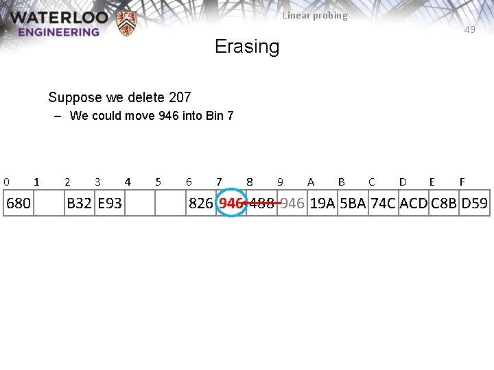
Linear probing 49 Erasing Suppose we delete 207 – We could move 946 into Bin 7 0 680 1 2 3 B 32 E 93 4 5 6 7 8 9 A B C D E F 826 946 488 946 19 A 5 BA 74 C ACD C 8 B D 59

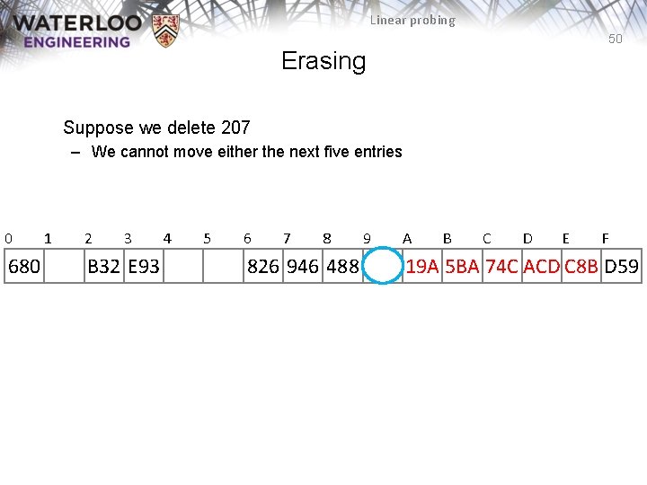
Linear probing 50 Erasing Suppose we delete 207 – We cannot move either the next five entries 0 680 1 2 3 B 32 E 93 4 5 6 7 8 826 946 488 9 A B C D E F 19 A 5 BA 74 C ACD C 8 B D 59

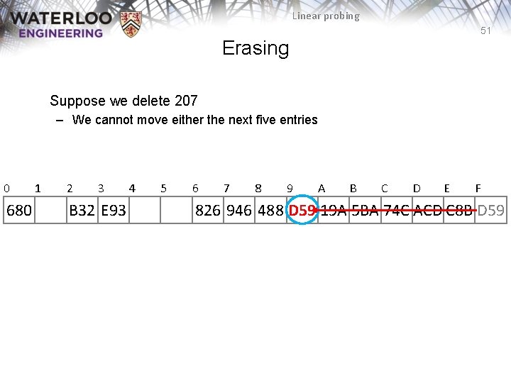
Linear probing 51 Erasing Suppose we delete 207 – We cannot move either the next five entries 0 680 1 2 3 B 32 E 93 4 5 6 7 8 9 A B C D E F 826 946 488 D 59 19 A 5 BA 74 C ACD C 8 B D 59

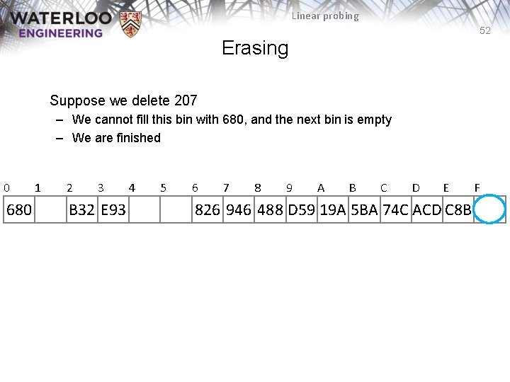
Linear probing 52 Erasing Suppose we delete 207 – We cannot fill this bin with 680, and the next bin is empty – We are finished 0 680 1 2 3 B 32 E 93 4 5 6 7 8 9 A B C D E 826 946 488 D 59 19 A 5 BA 74 C ACD C 8 B F

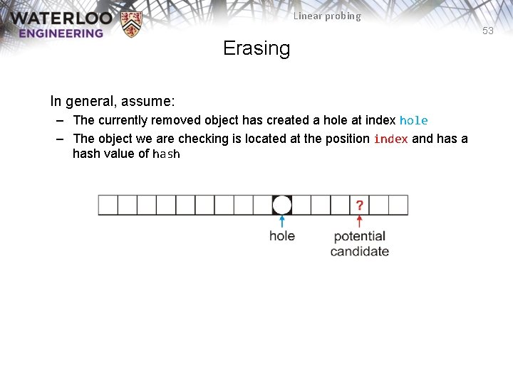
Linear probing 53 Erasing In general, assume: – The currently removed object has created a hole at index hole – The object we are checking is located at the position index and has a hash value of hash

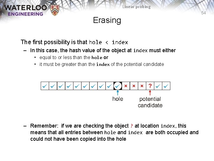
Linear probing 54 Erasing The first possibility is that hole < index – In this case, the hash value of the object at index must either • equal to or less than the hole or • it must be greater than the index of the potential candidate – Remember: if we are checking the object ? at location index, this means that all entries between hole and index are both occupied and could not have been copied into the hole

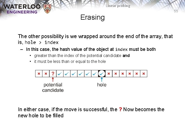
Linear probing 55 Erasing The other possibility is we wrapped around the end of the array, that is, hole > index – In this case, the hash value of the object at index must be both • greater than the index of the potential candidate and • it must be less than or equal to the hole In either case, if the move is successful, the ? Now becomes the new hole to be filled

Linear probing 56 Black Board Example Using the last digit as our hash function—insert these nine numbers into a hash table of size M = 10 31, 15, 79, 55, 42, 99, 60, 80, 23 Then, remove 79, 31, 42, and 60, in that order

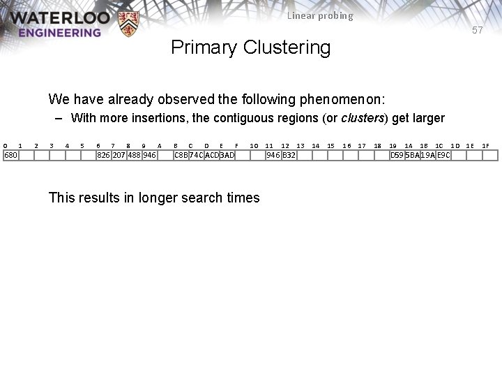
Linear probing 57 Primary Clustering We have already observed the following phenomenon: – With more insertions, the contiguous regions (or clusters) get larger 0 680 1 2 3 4 5 6 7 8 9 826 207 488 946 A B C D E F 10 C 8 B 74 C ACD 3 AD This results in longer search times 11 12 946 B 32 13 14 15 16 17 18 19 1 A 1 B 1 C D 59 5 BA 19 A E 9 C 1 D 1 E 1 F

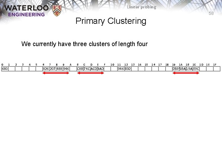
Linear probing 58 Primary Clustering We currently have three clusters of length four 0 680 1 2 3 4 5 6 7 8 9 826 207 488 946 A B C D E C 8 B 74 C ACD 3 AD F 10 11 12 946 B 32 13 14 15 16 17 18 19 1 A 1 B 1 C D 59 5 BA 19 A E 9 C 1 D 1 E 1 F

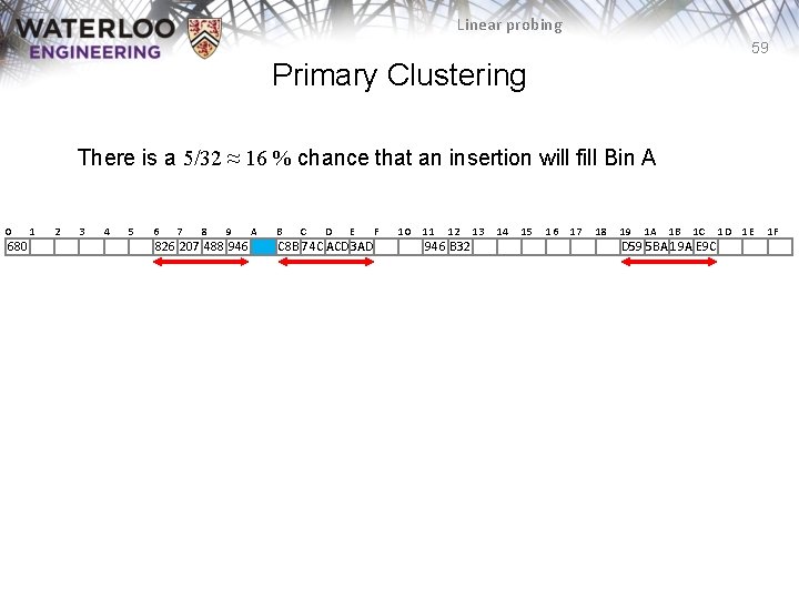
Linear probing 59 Primary Clustering There is a 5/32 ≈ 16 % chance that an insertion will fill Bin A 0 680 1 2 3 4 5 6 7 8 9 826 207 488 946 A B C D E C 8 B 74 C ACD 3 AD F 10 11 12 946 B 32 13 14 15 16 17 18 19 1 A 1 B 1 C D 59 5 BA 19 A E 9 C 1 D 1 E 1 F

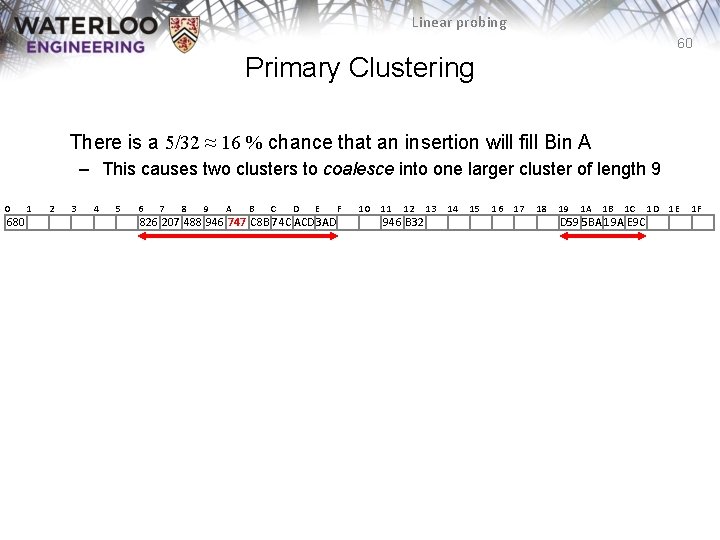
Linear probing 60 Primary Clustering There is a 5/32 ≈ 16 % chance that an insertion will fill Bin A – This causes two clusters to coalesce into one larger cluster of length 9 0 680 1 2 3 4 5 6 7 8 9 A B C D E 826 207 488 946 747 C 8 B 74 C ACD 3 AD F 10 11 12 946 B 32 13 14 15 16 17 18 19 1 A 1 B 1 C D 59 5 BA 19 A E 9 C 1 D 1 E 1 F

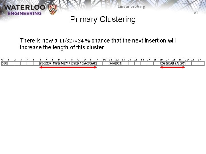
Linear probing 61 Primary Clustering There is now a 11/32 ≈ 34 % chance that the next insertion will increase the length of this cluster 0 680 1 2 3 4 5 6 7 8 9 A B C D E 826 207 488 946 747 C 8 B 74 C ACD 3 AD F 10 11 12 946 B 32 13 14 15 16 17 18 19 1 A 1 B 1 C D 59 5 BA 19 A E 9 C 1 D 1 E 1 F

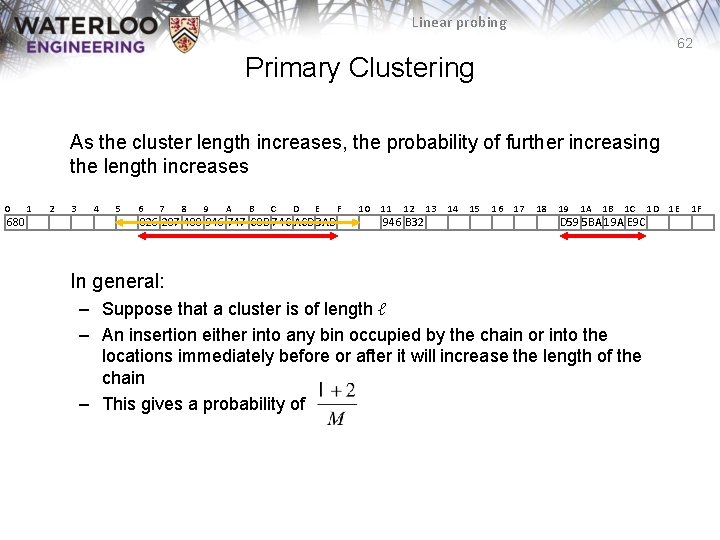
Linear probing 62 Primary Clustering As the cluster length increases, the probability of further increasing the length increases 0 680 1 2 3 4 5 6 7 8 9 A B C D E 826 207 488 946 747 C 8 B 74 C ACD 3 AD F 10 11 12 946 B 32 13 14 15 16 17 18 19 1 A 1 B 1 C D 59 5 BA 19 A E 9 C In general: – Suppose that a cluster is of length ℓ – An insertion either into any bin occupied by the chain or into the locations immediately before or after it will increase the length of the chain – This gives a probability of 1 D 1 E 1 F

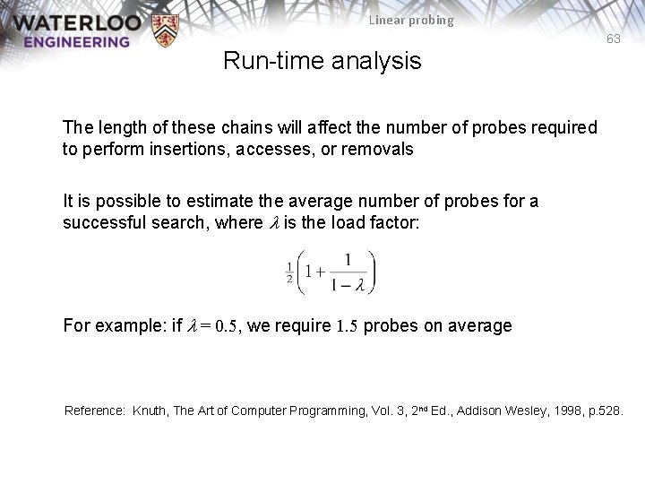
Linear probing 63 Run-time analysis The length of these chains will affect the number of probes required to perform insertions, accesses, or removals It is possible to estimate the average number of probes for a successful search, where l is the load factor: For example: if l = 0. 5, we require 1. 5 probes on average Reference: Knuth, The Art of Computer Programming, Vol. 3, 2 nd Ed. , Addison Wesley, 1998, p. 528.

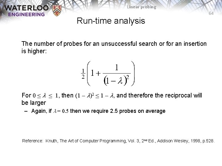
Linear probing 64 Run-time analysis The number of probes for an unsuccessful search or for an insertion is higher: For 0 ≤ l ≤ 1, then (1 – l)2 ≤ 1 – l, and therefore the reciprocal will be larger – Again, if l = 0. 5 then we require 2. 5 probes on average Reference: Knuth, The Art of Computer Programming, Vol. 3, 2 nd Ed. , Addison Wesley, 1998, p. 528.

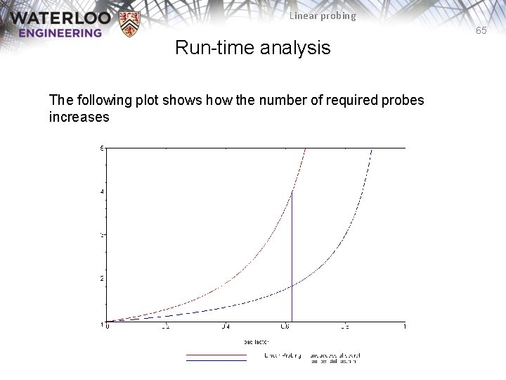
Linear probing 65 Run-time analysis The following plot shows how the number of required probes increases

Linear probing 66 Run-time analysis Our goal was to keep all operations Q(1) Unfortunate, as l grows, so does the run time One solution is to keep the load factor under a given bound If we choose l = 2/3, then the number of probes for either a successful or unsuccessful search is 2 and 5, respectively

Linear probing 67 Run-time analysis Therefore, we have three choices: – Choose M large enough so that we will not pass this load factor • This could waste memory – Double the number of bins if the chosen load factor is reached • Not available if dynamic memory allocation is not available – Choose a different strategy from linear probing • Two possibilities are quadratic probing and double hashing

Linear probing 68 Summary This topic introduced linear problem – – – Continue looking forward until an empty cell is found Searching follows the same rule Removing an object is more difficult Primary clustering is an issue Keep the load factor l ≤ 2/3

Linear probing 69 References Wikipedia, http: //en. wikipedia. org/wiki/Hash_function [1] [2] Cormen, Leiserson, and Rivest, Introduction to Algorithms, Mc. Graw Hill, 1990. Weiss, Data Structures and Algorithm Analysis in C++, 3 rd Ed. , Addison Wesley. These slides are provided for the ECE 250 Algorithms and Data Structures course. The material in it reflects Douglas W. Harder’s best judgment in light of the information available to him at the time of preparation. Any reliance on these course slides by any party for any other purpose are the responsibility of such parties. Douglas W. Harder accepts no responsibility for damages, if any, suffered by any party as a result of decisions made or actions based on these course slides for any other purpose than that for which it was intended.