EC 941 Game Theory Lecture 3 Francesco Squintani

EC 941 - Game Theory Lecture 3 Francesco Squintani Email: f. squintani@warwick. ac. uk 1

Structure of the Lecture n Bayesian Games and Nash Equilibrium n Bayesian Games and Information n Cournot Duopoly with Private Information n Public Good Provision with Private Information 2

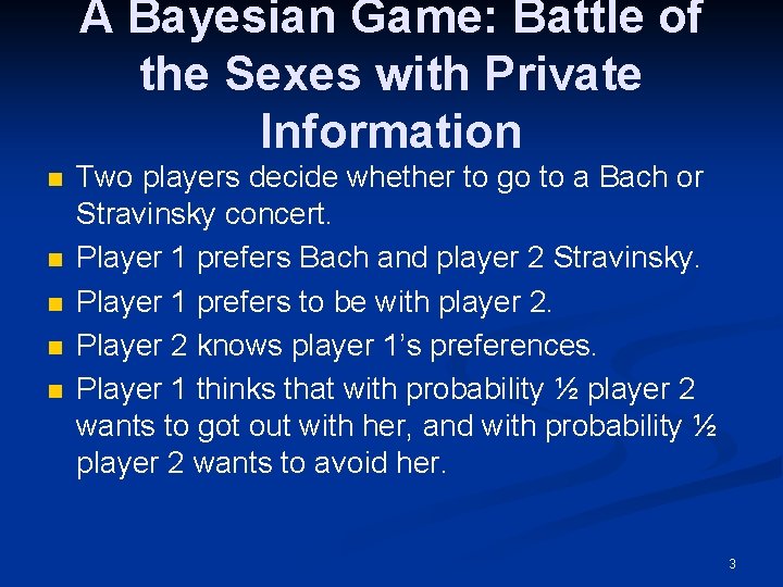
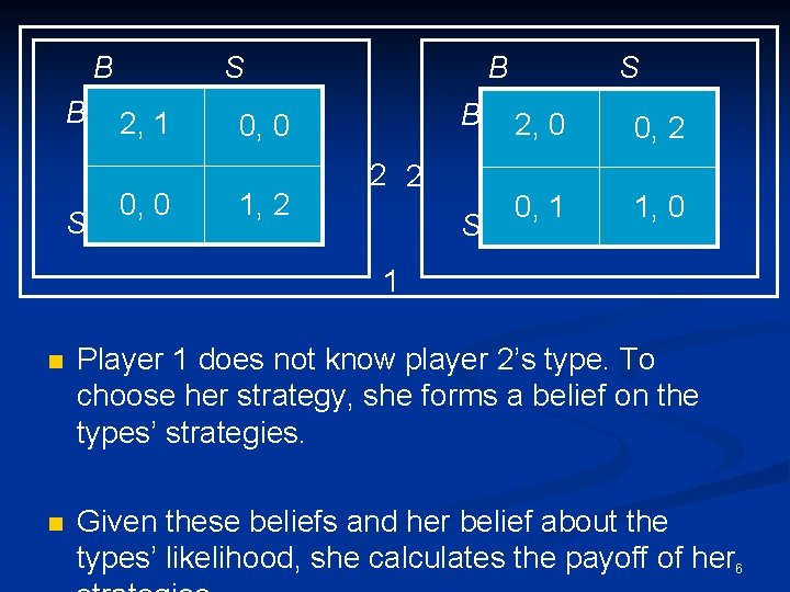
A Bayesian Game: Battle of the Sexes with Private Information n n Two players decide whether to go to a Bach or Stravinsky concert. Player 1 prefers Bach and player 2 Stravinsky. Player 1 prefers to be with player 2. Player 2 knows player 1’s preferences. Player 1 thinks that with probability ½ player 2 wants to got out with her, and with probability ½ player 2 wants to avoid her. 3

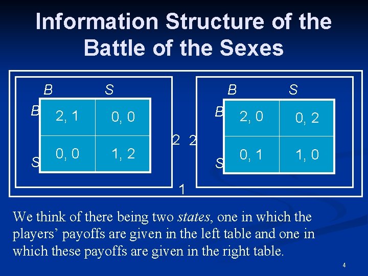
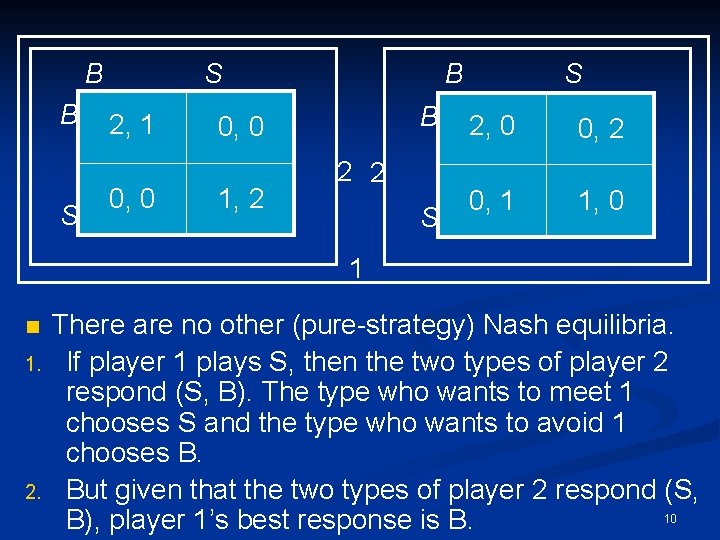
Information Structure of the Battle of the Sexes B B S S 2, 1 0, 0 B B 0, 0 1, 2 2 2 S S 2, 0 0, 2 0, 1 1, 0 1 We think of there being two states, one in which the players’ payoffs are given in the left table and one in which these payoffs are given in the right table. 4

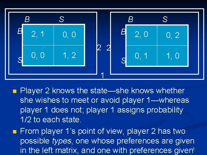
B B S S 2, 1 0, 0 B B 0, 0 1, 2 2 2 S S 2, 0 0, 2 0, 1 1, 0 1 n n Player 2 knows the state—she knows whether she wishes to meet or avoid player 1—whereas player 1 does not; player 1 assigns probability 1/2 to each state. From player 1’s point of view, player 2 has two possible types, one whose preferences are given in the left matrix, and one with preferences given 5

B B S S 2, 1 0, 0 B B 0, 0 1, 2 2 2 S S 2, 0 0, 2 0, 1 1, 0 1 n Player 1 does not know player 2’s type. To choose her strategy, she forms a belief on the types’ strategies. n Given these beliefs and her belief about the types’ likelihood, she calculates the payoff of her 6

Bayesian Nash Equilibrium of the Battle of the Sexes A Bayesian Nash equilibrium is a triple of strategies, one for player 1 and one for each type of player 2: 1. player 1’s strategy is optimal, given the strategies of the two types of player 2 and player 1’s beliefs on player 2’s type. 2. the strategy of each type of player 2 is optimal, given player 1’s strategy. 7

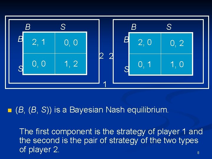
B B S S 2, 1 0, 0 B B 0, 0 1, 2 2 2 S S 2, 0 0, 2 0, 1 1, 0 1 n (B, S)) is a Bayesian Nash equilibrium. The first component is the strategy of player 1 and the second is the pair of strategy of the two types of player 2. 8

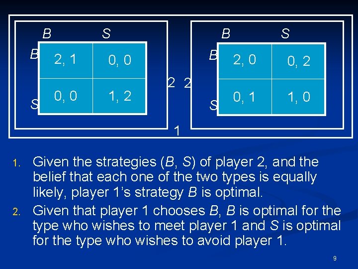
B B S S 2, 1 0, 0 B B 0, 0 1, 2 2 2 S S 2, 0 0, 2 0, 1 1, 0 1 1. 2. Given the strategies (B, S) of player 2, and the belief that each one of the two types is equally likely, player 1’s strategy B is optimal. Given that player 1 chooses B, B is optimal for the type who wishes to meet player 1 and S is optimal for the type who wishes to avoid player 1. 9

B B S S 2, 1 0, 0 B B 0, 0 1, 2 2 2 S S 2, 0 0, 2 0, 1 1, 0 1 n 1. 2. There are no other (pure-strategy) Nash equilibria. If player 1 plays S, then the two types of player 2 respond (S, B). The type who wants to meet 1 chooses S and the type who wants to avoid 1 chooses B. But given that the two types of player 2 respond (S, 10 B), player 1’s best response is B.

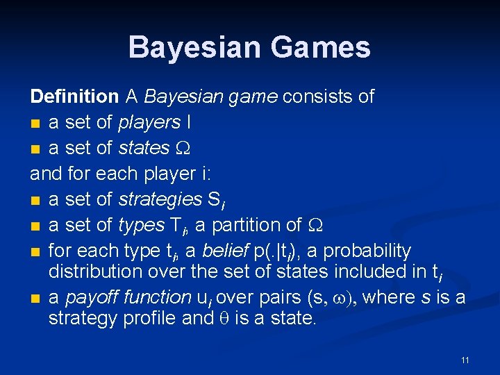
Bayesian Games Definition A Bayesian game consists of n a set of players I n a set of states W and for each player i: n a set of strategies Si n a set of types Ti, a partition of W n for each type ti, a belief p(. |ti), a probability distribution over the set of states included in ti n a payoff function ui over pairs (s, w), where s is a strategy profile and q is a state. 11

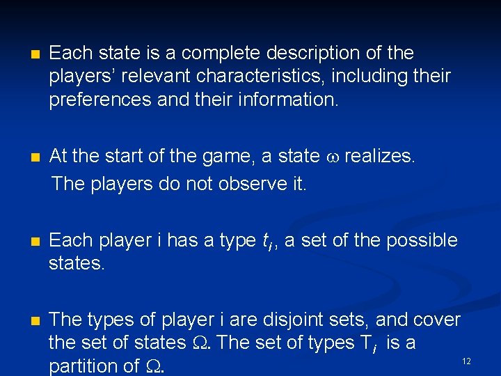
n n Each state is a complete description of the players’ relevant characteristics, including their preferences and their information. At the start of the game, a state w realizes. The players do not observe it. n Each player i has a type ti , a set of the possible states. n The types of player i are disjoint sets, and cover the set of states W. The set of types Ti is a 12 partition of W.

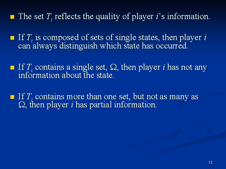
n The set Ti reflects the quality of player i’s information. n If Ti is composed of sets of single states, then player i can always distinguish which state has occurred. n n If Ti contains a single set, W, then player i has not any information about the state. If Ti contains more than one set, but not as many as W, then player i has partial information. 13

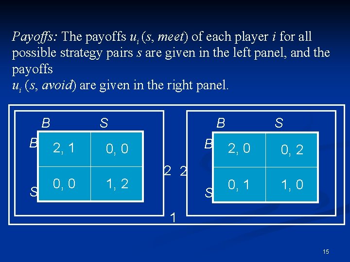
Battle of the Sexes n n n Players: The pair of people. States: The set of states is W ={meet, avoid}. Strategies: The strategies of each player are Si={B, S}. Types: Player 1 has a single type t 1= W. Player 2 has two types {meet} and {avoid}. Beliefs: Player 1 assigns probability 1/2 to each state. Player 2 knows the state. 14

Payoffs: The payoffs ui (s, meet) of each player i for all possible strategy pairs s are given in the left panel, and the payoffs ui (s, avoid) are given in the right panel. B B S S 2, 1 0, 0 B B 0, 0 1, 2 2 2 S S 2, 0 0, 2 0, 1 1, 0 1 15

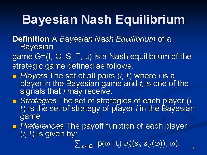
Bayesian Nash Equilibrium Definition A Bayesian Nash Equilibrium of a Bayesian game G=(I, W, S, T, u) is a Nash equilibrium of the strategic game defined as follows. n Players The set of all pairs (i, ti) where i is a player in the Bayesian game and ti is one of the signals that i may receive. n Strategies The set of strategies of each player (i, ti) is the set of strategy of player i in the Bayesian game. n Preferences The payoff function of each player (i, ti) is given by: ∑w∈W p(w | ti) ui((si, s-i (w)), w). 16

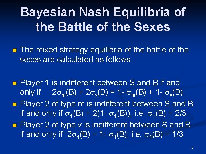
Bayesian Nash Equilibria of the Battle of the Sexes n The mixed strategy equilibria of the battle of the sexes are calculated as follows. n Player 1 is indifferent between S and B if and only if 2 sm(B) + 2 sv(B) = 1 - sm(B) + 1 - sv(B). Player 2 of type m is indifferent between S and B if and only if s 1(B) = 2(1 - s 1(B)), i. e. s 1(B) = 2/3. Player 2 of type v is indifferent between S and B if and only if 2 s 1(B) = 1 - s 1(B), i. e. s 1(B) = 1/3. n n 17

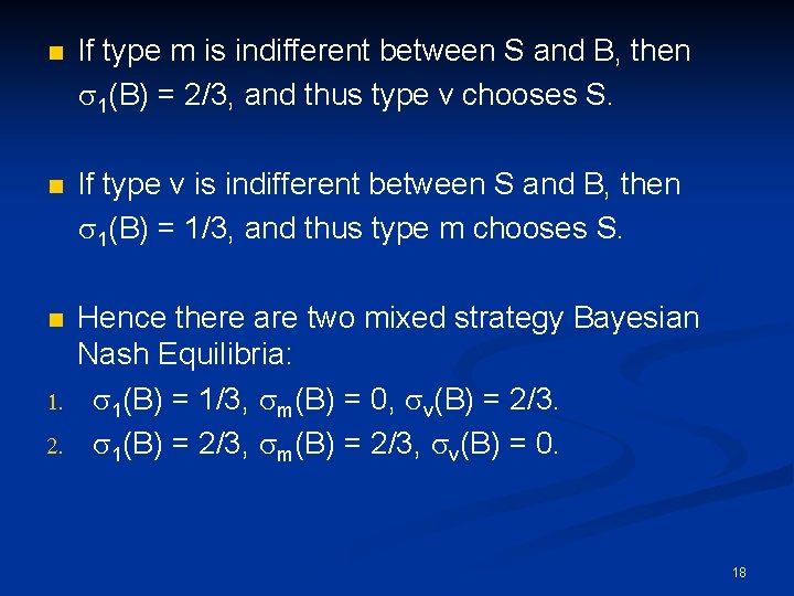
n If type m is indifferent between S and B, then s 1(B) = 2/3, and thus type v chooses S. n If type v is indifferent between S and B, then s 1(B) = 1/3, and thus type m chooses S. n Hence there are two mixed strategy Bayesian Nash Equilibria: s 1(B) = 1/3, sm(B) = 0, sv(B) = 2/3. s 1(B) = 2/3, sm(B) = 2/3, sv(B) = 0. 1. 2. 18

More Information May Hurt n A decision-maker in a single-person decision problem cannot be worse off if she has more information. If she wishes, she can ignore the information. n In a game, the same is not true: if a player has more information, and the other players know that she has more information, then she may be worse off. 19

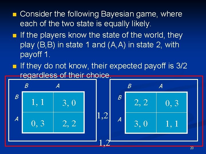
n n n Consider the following Bayesian game, where each of the two state is equally likely. If the players know the state of the world, they play (B, B) in state 1 and (A, A) in state 2, with payoff 1. If they do not know, their expected payoff is 3/2 regardless of their choice. B B A A 1, 1 0, 3 B B 3, 0 2, 2 1, 2 A A 2, 2 0, 3 3, 0 1, 1 20

Common Knowledge n There is a subtle difference between a situation in which all players know the payoffs, and a situation in which the payoffs are common knowledge. n When payoffs are common knowledge, all players know them, and know that all players know them and so on. n Lack of common knowledge may lead to players being unable to coordinate on the Pareto optimal 21

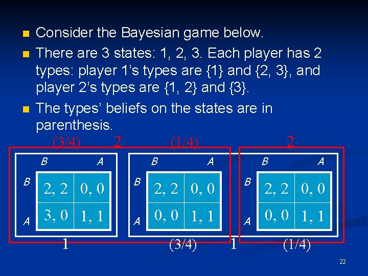
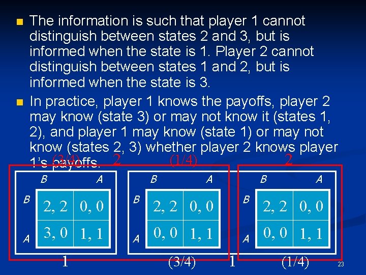
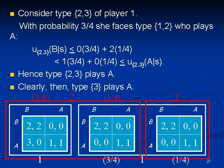
n n n Consider the Bayesian game below. There are 3 states: 1, 2, 3. Each player has 2 types: player 1’s types are {1} and {2, 3}, and player 2’s types are {1, 2} and {3}. The types’ beliefs on the states are in parenthesis. (3/4) 2 (1/4) 2 B B A A 2, 2 0, 0 3, 0 1, 1 1 B B A A B B 2, 2 0, 0 1, 1 (3/4) A 1 A 2, 2 0, 0 1, 1 (1/4) 22

n n The information is such that player 1 cannot distinguish between states 2 and 3, but is informed when the state is 1. Player 2 cannot distinguish between states 1 and 2, but is informed when the state is 3. In practice, player 1 knows the payoffs, player 2 may know (state 3) or may not know it (states 1, 2), and player 1 may know (state 1) or may not know (states 2, 3) whether player 2 knows player (3/4) 2 (1/4) 2 1’s payoffs. B B A A 2, 2 0, 0 3, 0 1, 1 1 B B A A B B 2, 2 0, 0 1, 1 (3/4) A 1 A 2, 2 0, 0 1, 1 (1/4) 23

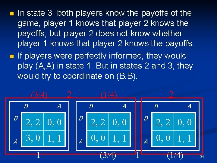
n n In state 3, both players know the payoffs of the game, player 1 knows that player 2 knows the payoffs, but player 2 does not know whether player 1 knows that player 2 knows the payoffs. If players were perfectly informed, they would play (A, A) in state 1. But in states 2 and 3, they would try to coordinate on (B, B). 2 (3/4) B B A A 2, 2 0, 0 3, 0 1, 1 1 2 (1/4) B B A A B B 2, 2 0, 0 1, 1 (3/4) A 1 A 2, 2 0, 0 1, 1 (1/4) 24

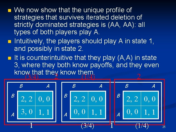
n n n We now show that the unique profile of strategies that survives iterated deletion of strictly dominated strategies is (AA, AA): all types of both players play A. Intuitively, the players should play A in state 1, and possibly in state 2. It is counterintuitive that they play (A, A) in state 3, where they both know payoffs, and they even know that they know them. (3/4) 2 (1/4) 2 B B A A 2, 2 0, 0 3, 0 1, 1 1 B B A A B B 2, 2 0, 0 1, 1 (3/4) A 1 A 2, 2 0, 0 1, 1 (1/4) 25

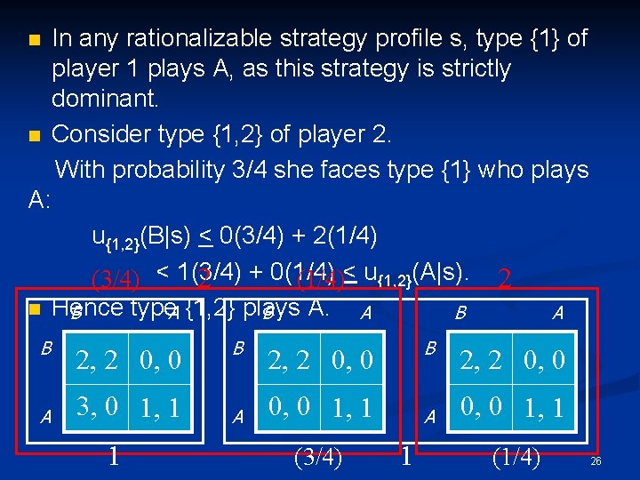
n n In any rationalizable strategy profile s, type {1} of player 1 plays A, as this strategy is strictly dominant. Consider type {1, 2} of player 2. With probability 3/4 she faces type {1} who plays A: n B A u{1, 2}(B|s) < 0(3/4) + 2(1/4) (3/4) < 1(3/4) 2 + 0(1/4)< u{1, 2}(A|s). Hence type. A {1, 2} plays A. A B B B 2, 2 0, 0 3, 0 1, 1 1 B A B 2, 2 0, 0 1, 1 (3/4) A 1 2 A 2, 2 0, 0 1, 1 (1/4) 26

n Consider type {2, 3} of player 1. With probability 3/4 she faces type {1, 2} who plays A: n n u{2, 3}(B|s) < 0(3/4) + 2(1/4) < 1(3/4) + 0(1/4) < u{2, 3}(A|s). Hence type {2, 3} plays A. Clearly, then, type {3} plays A. (3/4) 2 (1/4) B B A A 2, 2 0, 0 3, 0 1, 1 1 B B A A B B 2, 2 0, 0 1, 1 (3/4) 2 A 1 A 2, 2 0, 0 1, 1 (1/4) 27

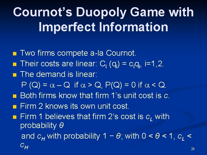
Cournot’s Duopoly Game with Imperfect Information n n n Two firms compete a-la Cournot. Their costs are linear: Ci (qi) = ciqi, i=1, 2. The demand is linear: P (Q) = a – Q if a > Q, P(Q) = 0 if a < Q. Both firms know that firm 1’s unit cost is c. Firm 2 knows its own unit cost. Firm 1 believes that firm 2’s cost is c. L with probability θ and c. H with probability 1 − θ; with 0 < θ < 1, c. L < c. H. 28

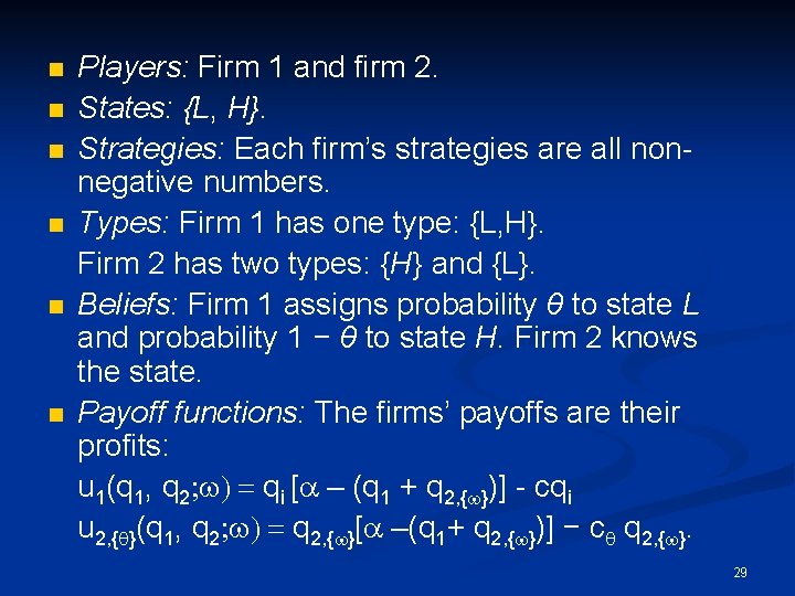
n n n Players: Firm 1 and firm 2. States: {L, H}. Strategies: Each firm’s strategies are all nonnegative numbers. Types: Firm 1 has one type: {L, H}. Firm 2 has two types: {H} and {L}. Beliefs: Firm 1 assigns probability θ to state L and probability 1 − θ to state H. Firm 2 knows the state. Payoff functions: The firms’ payoffs are their profits: u 1(q 1, q 2; w) = qi [a – (q 1 + q 2, {w})] - cqi u 2, {q}(q 1, q 2; w) = q 2, {w}[a –(q 1+ q 2, {w})] − cq q 2, {w}. 29

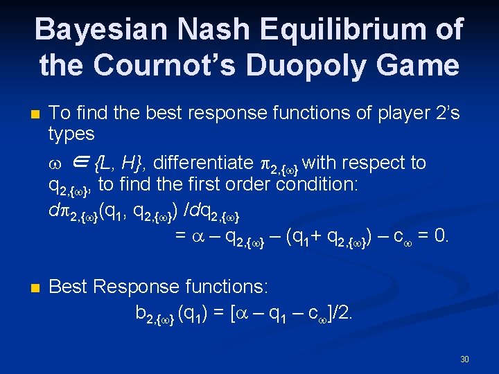
Bayesian Nash Equilibrium of the Cournot’s Duopoly Game n To find the best response functions of player 2’s types w ∈ {L, H}, differentiate p 2, {w} with respect to q 2, {w}, to find the first order condition: dp 2, {w}(q 1, q 2, {w}) /dq 2, {w} = a – q 2, {w} – (q 1+ q 2, {w}) – cw = 0. n Best Response functions: b 2, {w} (q 1) = [a – q 1 – cw]/2. 30

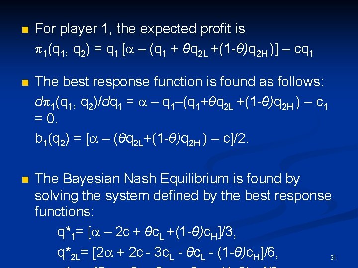
n For player 1, the expected profit is p 1(q 1, q 2) = q 1 [a – (q 1 + θq 2 L +(1 -θ)q 2 H )] – cq 1 n The best response function is found as follows: dp 1(q 1, q 2)/dq 1 = a – q 1–(q 1+θq 2 L +(1 -θ)q 2 H ) – c 1 = 0. b 1(q 2) = [a – (θq 2 L+(1 -θ)q 2 H ) – c]/2. n The Bayesian Nash Equilibrium is found by solving the system defined by the best response functions: q*1= [a – 2 c + θc. L +(1 -θ)c. H]/3, q*2 L= [2 a + 2 c - 3 c. L - θc. L - (1 -θ)c. H]/6, 31

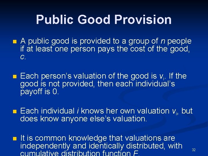
Public Good Provision n A public good is provided to a group of n people if at least one person pays the cost of the good, c. n Each person’s valuation of the good is vi. If the good is not provided, then each individual’s payoff is 0. n Each individual i knows her own valuation vi, but does know anyone else’s valuation. n It is common knowledge that valuations are independently and identically distributed, with 32

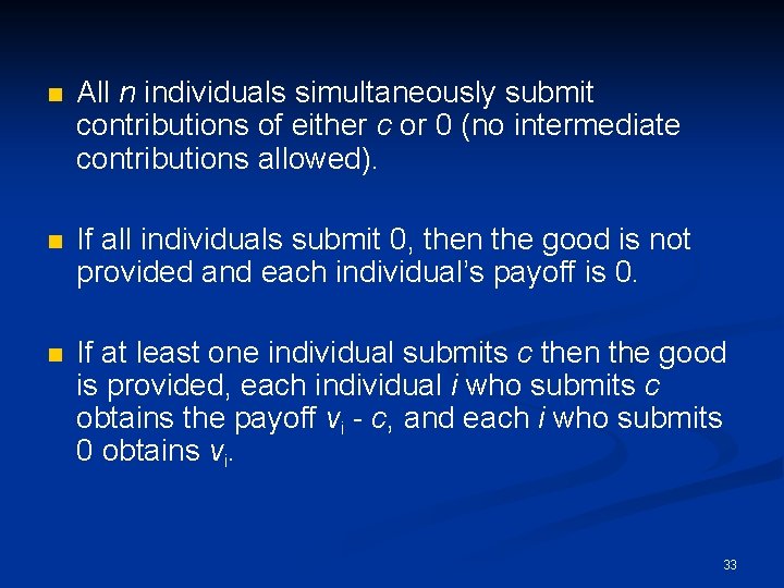
n All n individuals simultaneously submit contributions of either c or 0 (no intermediate contributions allowed). n If all individuals submit 0, then the good is not provided and each individual’s payoff is 0. n If at least one individual submits c then the good is provided, each individual i who submits c obtains the payoff vi - c, and each i who submits 0 obtains vi. 33

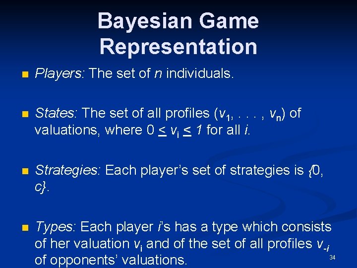
Bayesian Game Representation n Players: The set of n individuals. n States: The set of all profiles (v 1, . . . , vn) of valuations, where 0 < vi < 1 for all i. n Strategies: Each player’s set of strategies is {0, c}. n Types: Each player i’s has a type which consists of her valuation vi and of the set of all profiles v-i 34 of opponents’ valuations.

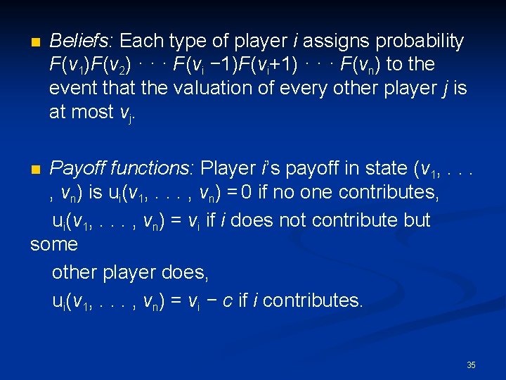
n Beliefs: Each type of player i assigns probability F(v 1)F(v 2) · · · F(vi − 1)F(vi+1) · · · F(vn) to the event that the valuation of every other player j is at most vj. Payoff functions: Player i’s payoff in state (v 1, . . . , vn) is ui(v 1, . . . , vn) = 0 if no one contributes, ui(v 1, . . . , vn) = vi if i does not contribute but some other player does, ui(v 1, . . . , vn) = vi − c if i contributes. n 35

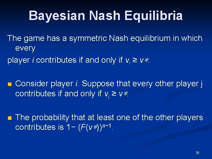
Bayesian Nash Equilibria The game has a symmetric Nash equilibrium in which every player i contributes if and only if vi ≥ v∗. n Consider player i. Suppose that every other player j contributes if and only if vj ≥ v∗. n The probability that at least one of the other players contributes is 1− (F(v∗))n− 1. 36

n Player i’s expected payoff is [1 − (F(v∗))n− 1] vi if she does not contribute and vi − c if she contributes. n The conditions for player i to not contribute when vi < v∗ and contribute when vi ≥ v∗ are: (1−(F(v∗))n− 1)vi > vi−c if vi< v∗, (1−(F(v∗))n− 1)vi ≤ vi−c if vi ≥ v∗: I. e. vi(F(v∗))n− 1 < c if vi < v∗, v∗. n i (F(v v ∗))n− 1 ≥ c if vi ≥ Hence, in equilibrium, v∗(F(v∗))n− 1 = c. 37

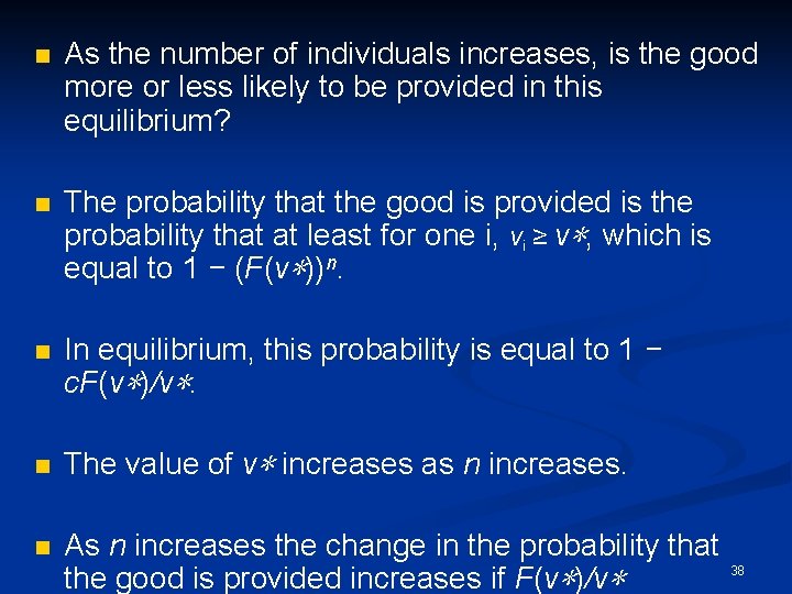
n As the number of individuals increases, is the good more or less likely to be provided in this equilibrium? n The probability that the good is provided is the probability that at least for one i, vi ≥ v∗, which is equal to 1 − (F(v∗))n. n In equilibrium, this probability is equal to 1 − c. F(v∗)/v∗. n The value of v∗ increases as n increases. n As n increases the change in the probability that the good is provided increases if F(v∗)/v∗ 38

Summary of the Lecture n Bayesian Games and Nash Equilibrium n Bayesian Games and Information n Cournot Duopoly with Private Information n Public Good Provision with Private Information 39

Preview of the Next Lecture n Juries and Information Aggregation n Auctions with Private Information 40