EAT 453 ADVANCED STRUCTURAL ANALYSIS LECTURE 2 FUNDAMENTALS

EAT 453 ADVANCED STRUCTURAL ANALYSIS LECTURE 2 FUNDAMENTALS FOR FINITE ELEMENT METHOD ILYA BINTI JOOHARI

TOPICS § The Hamilton’s Principle § The finite element procedure § Domain Discretization § Displacement Interpolation § Shape Functions § Coordinate Transformation § Assembly of Global FE equation

FINITE ELEMENT METHOD (FEM) § The FEM was first used to solve problems of stress analysis, and has since been applied to many other problems like thermal analysis, fluid flow analysis, piezoelectric analysis, and many others. § Basically, the analyst seeks to determine the distribution of some field variable like the displacement in stress analysis, the temperature or heat flux in thermal analysis, the electrical charge in electrical analysis, and so on. § The FEM is a numerical method seeking an approximated solution of the distribution of field variables in the problem domain that is difficult to obtain analytically. § It is done by dividing the problem domain into several elements.

Fixed boundary uniform loading Finite element Cantilever plate model in plane strain • Approximate method • Geometric model Element • Node • Element • Mesh • Discretization Node Problem: Obtain the stresses/strains in the plate

INTRODUCTION § When using the Finite Element Method (FEM) to solve mechanics problems, the domain is first discretized into small elements. § In each of these elements, the profile of the displacements is assumed in simple forms to obtain element equations. § The equations obtained for each element are then assembled together with adjoining elements to form the global finite element equation for the whole problem domain. § Equations thus created for the global problem domain can be solved easily for the entire displacement field.

THE HAMILTON’S PRINCIPLE § Hamilton’s principle is a simple yet powerful tool that can be used to derive discretized dynamic system equations. It states simply that “Of all the admissible time histories of displacement the most accurate solution makes the Lagrangian functional a minimum. ”

THE HAMILTON’S PRINCIPLE (cont. ) § An admissible displacement must satisfy the following conditions: (a) the compatibility equations, (b) the essential or the kinematic boundary conditions, and (c) the conditions at initial (t 1) and final time (t 2) § Condition (a) ensures that the displacements are compatible (continuous) in the problem domain. § Condition (b) ensures that the displacement constraints are satisfied. § Condition (c) requires the displacement history to satisfy the constraints at the initial and final times.

THE HAMILTON’S PRINCIPLE (cont. ) § Mathematically, Hamilton’s principle states: § The Langrangian functional, L, is obtained using a set of admissible time histories of displacements, and it consists of § T is the kinetic energy § �is the potential energy (i. e. elastic strain energy) § Wf is the work done by the external forces.

THE HAMILTON’S PRINCIPLE (cont. ) § The kinetic energy of the entire problem domain is defined in the integral form § V represents the whole volume of the solid § U is the set of admissible time histories of displacements § The strain energy in the entire domain of elastic solids and structures can be expressed as § where ε are the strains obtained using the set of admissible time histories of displacements

THE HAMILTON’S PRINCIPLE (cont. ) § The work done by the external forces over the set of admissible time histories of displacements can be obtained by § Sf represents the surface of the solid on which the surface forces are prescribed

ADVANTAGES OF THE HAMILTON’S PRINCIPLE § Hamilton’s principle allows one to simply assume any set of displacements, as long as it satisfies the three admissible conditions. § The power of Hamilton’s principle is that it provides the freedom of choice, opportunity and possibility. § For practical engineering problems, one usually does not have to pursue the exact solution, which in most cases are usually unobtainable, because we now have a choice to quite conveniently obtain a good approximation using Hamilton’s principle, by assuming the likely form, pattern or shape of the solutions. § Hamilton’s principle thus provides the foundation for the finite element methods.

ADVANTAGES OF THE HAMILTON’S PRINCIPLE § Furthermore, the simplicity of Hamilton’s principle manifests itself in the use of scalar energy quantities. § Engineers and scientists like working with scalar quantities when it comes to numerical calculations, as they do not need to worry about the direction. § All the mathematical tools required to derive the final discrete system equations are then basic integration, differentiation and variation, all of which are standard linear operations. § Another plus point of Hamilton’s principle is that the final discrete system equations produced are usually a set of linear algebraic equations that can be solved using conventional methods and standard computational routines.

FEM PROCEDURE

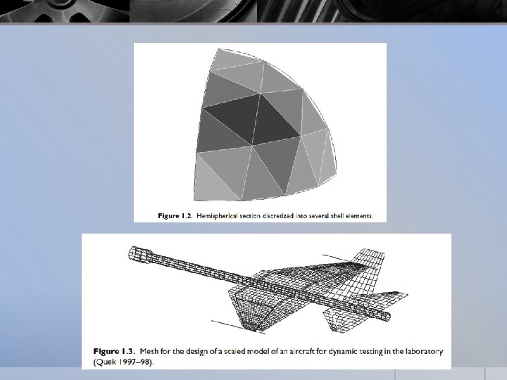
DOMAIN DISCRETIZATION § The solid body is divided into Ne elements. § The procedure is often called meshing, which is usually performed using so-called pre-processors. § This is especially true for complex geometries. § Figure shows an example of a mesh for a two dimensional solid.

DOMAIN DISCRETIZATION (cont. ) § The pre-processor generates unique numbers for all the elements and nodes for the solid or structure in a proper manner. § An element is formed by connecting its nodes in a pre-defined consistent fashion to create the connectivity of the element. § All the elements together form the entire domain of the problem without any gap or overlapping. § It is possible for the domain to consist of different types of elements with different numbers of nodes, as long as they are compatible (no gaps and overlapping; the admissible condition (a) required by Hamilton’s principle) on the boundaries between different elements.

DOMAIN DISCRETIZATION (cont. )

DOMAIN DISCRETIZATION (cont. ) § The density of the mesh depends upon the accuracy requirement of the analysis and the computational resources available. § Generally, a finer mesh will yield results that are more accurate, but will increase the computational cost. § As such, the mesh is usually not uniform, with a finer mesh being used in the areas where the displacement gradient is larger or where the accuracy is critical to the analysis. § The purpose of the domain discretization is to make it easier in assuming the pattern of the displacement field.

DISPLACEMENT INTERPOLATION § The FEM formulation has to be based on a coordinate system. § It is often convenient to use a local coordinate system that is defined for an element in reference to the global coordination system that is usually defined for structure, as shown. the entire

DISPLACEMENT INTERPOLATION (cont. ) § Based on the local coordinate system defined on an element, the displacement within the element is now assumed simply by polynomial interpolation using the displacements at its nodes (or nodal displacements)as § h § nd § di = approximation = the number of nodes forming the element § N = = the nodal displacement at the ith node, which is the unknown the analyst wants to compute matrix of shape function for the nodes in the element

DISPLACEMENT INTERPOLATION (cont. ) § nf is the number of Degrees Of Freedom (DOF) at a node. For 3 D solids, nf = 3 § The vector de is the displacement vector for the entire element,

DISPLACEMENT INTERPOLATION (cont. ) § The total DOF for the entire element is § N is a matrix of shape functions for the nodes in the element, which are predefined to assume the shapes of the displacement variations with respect to the coordinates. It has the general form of § where Ni arranged as is a sub-matrix of shape functions for displacement components, which is

SHAPE FUNCTIONS § Consider an element with nd node at § Where; § 1 Dimensional § 2 Dimensional § 3 Dimensional § First, the displacement component is approximated in the form of a linear combination of nd linearly-independent basis functions pi (x) Upi(x) - (equation 1) �i (x) - the approximation of the displacement component the basis function of monomials in the space coordinates x the coefficient for the monomial pi(x)

SHAPE FUNCTIONS (cont. ) § Vector � is defined as

SHAPE FUNCTIONS (cont. ) § The basis of complete order of p § One dimensional domain § Two dimensional domain § Three dimensional domain

SHAPE FUNCTIONS (cont. ) § de is the vector that includes the values of the displacement component at all the nd nodes in the element § and P is given by

SHAPE FUNCTIONS (cont. ) § Assuming that the inverse of the moment matrix P exists, (equation 2) § Substituting eq. 2 into eq. 1, we obtain § Or in matrix form

SHAPE FUNCTIONS (cont. ) § Where N(x) is a matrix of shape functions Ni(x) defined by

COORDINATE TRANSFORMATION § In general, the structure is divided into many elements with different orientations (see Figure). § To assemble all the element equations to form the coordinate global system transformation equations, has to a be performed for each element in order to formulate its element equation in reference to the global coordinate system which is defined on the whole structure.

COORDINATE TRANSFORMATION (cont. ) § The coordinate transformation gives the relationship between the displacement vector de based on the local coordinate system and the displacement vector De for the same element, but based on the global coordinate system: (equation 1) T is the transformation matrix § The transformation matrix can also be applied to the force vectors between the local and global coordinate systems: Fe stands for the force vector at node i on the global coordinate system.

COORDINATE TRANSFORMATION (cont. ) (equation 2) § Substituting eq 1 into eq 2, leads to the element equation based on the global coordinate system: § Where

ASSEMBLY OF GLOBAL FE EQUATION § The FE equations for all the individual elements can be assembled together to form the global FE system equation: § Where § K and M are the globe stiffness and mass matrix § D is a vector of all the displacements at all the nodes in the entire problem domain § F is a vector of all the equivalent nodal force vectors.

FEM FOR BEAMS

1. Shape Function Construction L = 2 a § As there are four DOFs for a beam element, there should be four shape functions. § It is often more convenient if the shape functions are derived from a special set of local coordinates, which is commonly known as the natural coordinate system. § This natural coordinate system has its origin at the centre of the element, and the element is defined from -1 to+1.

1. Shape Function Construction (cont. ) § The relationship between the natural coordinate system and the local coordinate system can be simply given as Equation 1 § The displacement in an element is first assumed in the form of a third order polynomial of ξ that contains four unknown constants: Equation 2 § Where � 0 to � 3 are the four unknown constants.

1. Shape Function Construction (cont. ) § The equation can have the following matrix form: or § Equation 3 The rotation θ can be obtained from the differential of Eq. 2 with the use of Eq. 1:

1. Shape Function Construction (cont. ) § The four unknown constants � 0 to � 3 can be determined by utilizing the following four conditions: § The application of the above four conditions gives Equation 4

1. Shape Function Construction (cont. ) § Where § Substituting Eq. 4 into Eq. 3 § where N is a matrix of shape functions given by

2. Strain Matrix § The relationship between normal strain and deflection § Which gives the relationship between the strain and the deflection, we have: § Where the strain matrix B is given by Equation 5 Assignment

3. Element Matrices § The stiffness matrix can be obtained as Equation 6 § Where is the second moment of area (or moment of inertia) of the cross-section of the beam with respect to the z axis.

3. Element Matrices (cont. ) § Substituting Eq. 5 into Eq. 6, we obtain stiffness matrix Equation 7

3. Element Matrices (cont. ) § To obtain the mass matrix,

Example: A uniform cantilever beam subjected to a downward force Consider the cantilever beam as shown below. The beam is fixed at one end, and it has a uniform cross-sectional area as shown. The beam undergoes static deflection by a downward load of P = 1000 N applied at the free end. The dimensions of the beam are shown in the figure, and the beam is made of aluminium whose properties are shown in Table. L = 2 a

Step 1: Obtaining the element matrices The beam element would have degrees of freedom as shown in figure below. The element stiffness matrix can be obtained using Eq. 7. Note that as this is a static problem, the mass matrix is not required here. The second moment of area of the cross-sectional area about the z-axis can be given as

Step 1: Obtaining the element matrices Since only one element is used, the stiffness matrix of the beam is thus the same as the element stiffness matrix:

Step 1: Obtaining the element matrices The finite element equation becomes F = KD

Step 2: Applying boundary conditions The beam is fixed at one end. Therefore, The reduced stiffness matrix becomes a 2 × 2 matrix of

Step 3: Solving the FE matrix equation The finite element equation, after the imposition of the displacement condition, is thus Where The force vector F is given as By using simultaneous equation

Step 3: Solving the FE matrix equation After v 2 and θ 2 have been obtained, they are substituted back into the first two equations to obtain the reaction shear force at node 1: and the reaction moment at node 1:

END