Eastern Mediterranean University Department of Industrial Engineering COURSE

Eastern Mediterranean University Department of Industrial Engineering COURSE: IENG 212 Modelling and Optimization Semester: Fall 2017 -2018 Name Of the Presentation: Transportation Problems Submitted by: OKAN CAN Student No: 133375 Group: 01

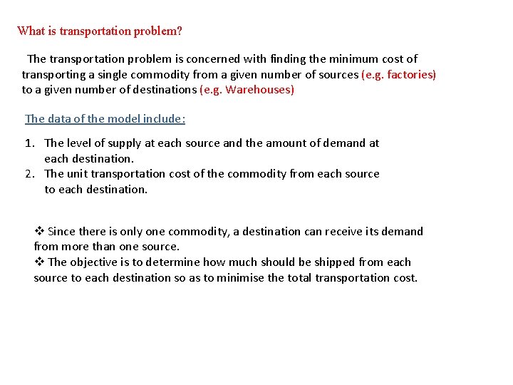
What is transportation problem? The transportation problem is concerned with finding the minimum cost of transporting a single commodity from a given number of sources (e. g. factories) to a given number of destinations (e. g. Warehouses) The data of the model include: 1. The level of supply at each source and the amount of demand at each destination. 2. The unit transportation cost of the commodity from each source to each destination. v Since there is only one commodity, a destination can receive its demand from more than one source. v The objective is to determine how much should be shipped from each source to each destination so as to minimise the total transportation cost.

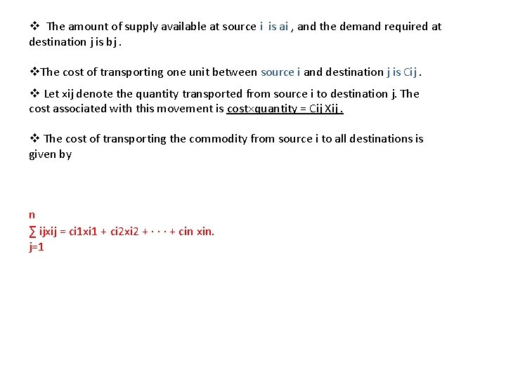
v The amount of supply available at source i is ai , and the demand required at destination j is bj. v. The cost of transporting one unit between source i and destination j is Cij. v Let xij denote the quantity transported from source i to destination j. The cost associated with this movement is cost×quantity = Cij Xij. v The cost of transporting the commodity from source i to all destinations is given by n ∑ ijxij = ci 1 xi 1 + ci 2 xi 2 + · · · + cin xin. j=1

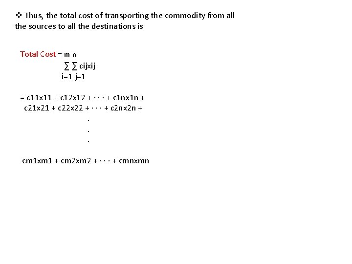
v Thus, the total cost of transporting the commodity from all the sources to all the destinations is Total Cost = m n ∑ ∑ cijxij i=1 j=1 = c 11 x 11 + c 12 x 12 + · · · + c 1 nx 1 n + c 21 x 21 + c 22 x 22 + · · · + c 2 nx 2 n + . cm 1 xm 1 + cm 2 xm 2 + · · · + cmnxmn

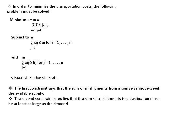
v In order to minimise the transportation costs, the following problem must be solved: Minimise z = m n ∑ ∑ cijxij , i=1 j=1 Subject to n ∑ xij ≤ ai for i = 1, . . . , m j=1 and m ∑ xij ≥ bj for j = 1, . . . , n i=1 where xij ≥ 0 for all i and j. v The first constraint says that the sum of all shipments from a source cannot exceed the available supply. v The second constraint specifies that the sum of all shipments to a destination must be at least as large as the demand.

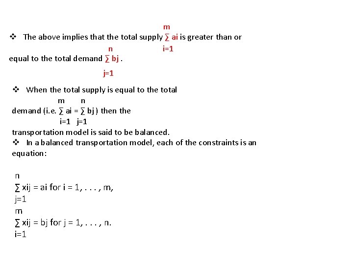
m v The above implies that the total supply ∑ ai is greater than or n i=1 equal to the total demand ∑ bj. j=1 v When the total supply is equal to the total m n demand (i. e. ∑ ai = ∑ bj ) then the i=1 j=1 transportation model is said to be balanced. v In a balanced transportation model, each of the constraints is an equation: n ∑ xij = ai for i = 1, . . . , m, j=1 m ∑ xij = bj for j = 1, . . . , n. i=1

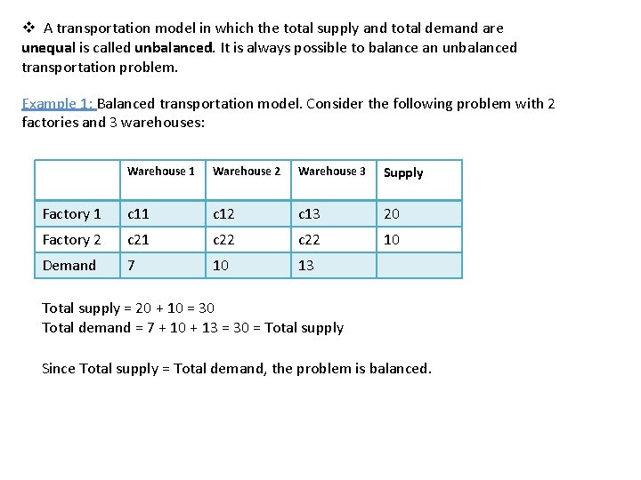
v A transportation model in which the total supply and total demand are unequal is called unbalanced. It is always possible to balance an unbalanced transportation problem. Example 1: Balanced transportation model. Consider the following problem with 2 factories and 3 warehouses: Warehouse 1 Warehouse 2 Warehouse 3 Supply Factory 1 c 12 c 13 20 Factory 2 c 21 c 22 10 Demand 7 10 13 Total supply = 20 + 10 = 30 Total demand = 7 + 10 + 13 = 30 = Total supply Since Total supply = Total demand, the problem is balanced.

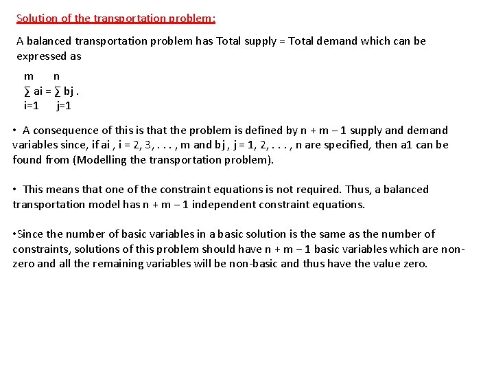
Solution of the transportation problem: A balanced transportation problem has Total supply = Total demand which can be expressed as m n ∑ ai = ∑ bj. i=1 j=1 • A consequence of this is that the problem is defined by n + m − 1 supply and demand variables since, if ai , i = 2, 3, . . . , m and bj , j = 1, 2, . . . , n are specified, then a 1 can be found from (Modelling the transportation problem). • This means that one of the constraint equations is not required. Thus, a balanced transportation model has n + m − 1 independent constraint equations. • Since the number of basic variables in a basic solution is the same as the number of constraints, solutions of this problem should have n + m − 1 basic variables which are nonzero and all the remaining variables will be non-basic and thus have the value zero.

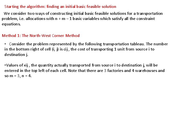
Starting the algorithm: finding an initial basic feasible solution We consider two ways of constructing initial basic feasible solutions for a transportation problem, i. e. allocations with n + m − 1 basic variables which satisfy all the constraint equations. Method 1: The North-West Corner Method • Consider the problem represented by the following transportation tableau. The number in the bottom right of cell (i, j) is cij , the cost of transporting 1 unit from source i to destination j. • Values of xij , the quantity actually transported from source i to destination j, will be entered in the top left of each cell. Note that there are 3 factories and 4 warehouses and so m = 3, n = 4.

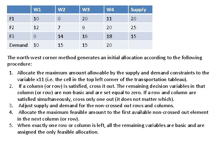
W 1 W 2 W 3 W 4 Supply F 1 10 0 20 11 20 F 2 12 7 9 20 25 F 3 0 14 16 18 15 Demand 10 15 15 20 The north-west corner method generates an initial allocation according to the following procedure: 1. Allocate the maximum amount allowable by the supply and demand constraints to the variable x 11 (i. e. the cell in the top left corner of the transportation tableau). 2. If a column (or row) is satisfied, cross it out. The remaining decision variables in that column (or row) are non-basic and are set equal to zero. If a row and column are satisfied simultaneously, cross only one out (it does not matter which). 3. Adjust supply and demand for the non-crossed out rows and columns. 4. Allocate the maximum feasible amount to the first available non-crossed out element in the next column (or row). 5. When exactly one row or column is left, all the remaining variables are basic and are assigned the only feasible allocation.

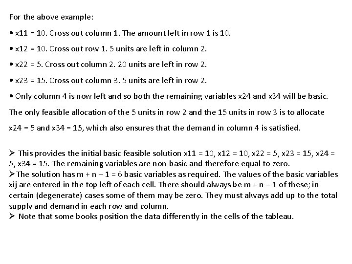
For the above example: • x 11 = 10. Cross out column 1. The amount left in row 1 is 10. • x 12 = 10. Cross out row 1. 5 units are left in column 2. • x 22 = 5. Cross out column 2. 20 units are left in row 2. • x 23 = 15. Cross out column 3. 5 units are left in row 2. • Only column 4 is now left and so both the remaining variables x 24 and x 34 will be basic. The only feasible allocation of the 5 units in row 2 and the 15 units in row 3 is to allocate x 24 = 5 and x 34 = 15, which also ensures that the demand in column 4 is satisfied. Ø This provides the initial basic feasible solution x 11 = 10, x 12 = 10, x 22 = 5, x 23 = 15, x 24 = 5, x 34 = 15. The remaining variables are non-basic and therefore equal to zero. ØThe solution has m + n − 1 = 6 basic variables as required. The values of the basic variables xij are entered in the top left of each cell. There should always be m + n − 1 of these; in certain (degenerate) cases some of them may be zero. They must always add up to the total supply and demand in each row and column. Ø Note that some books position the data differently in the cells of the tableau.

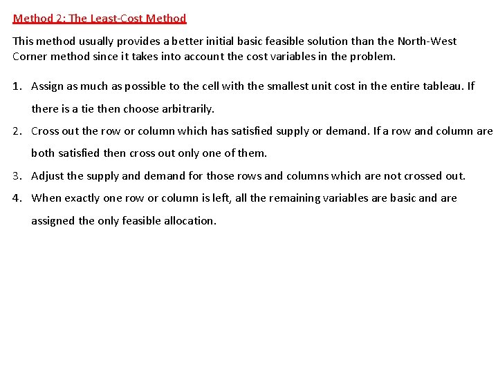
Method 2: The Least-Cost Method This method usually provides a better initial basic feasible solution than the North-West Corner method since it takes into account the cost variables in the problem. 1. Assign as much as possible to the cell with the smallest unit cost in the entire tableau. If there is a tie then choose arbitrarily. 2. Cross out the row or column which has satisfied supply or demand. If a row and column are both satisfied then cross out only one of them. 3. Adjust the supply and demand for those rows and columns which are not crossed out. 4. When exactly one row or column is left, all the remaining variables are basic and are assigned the only feasible allocation.

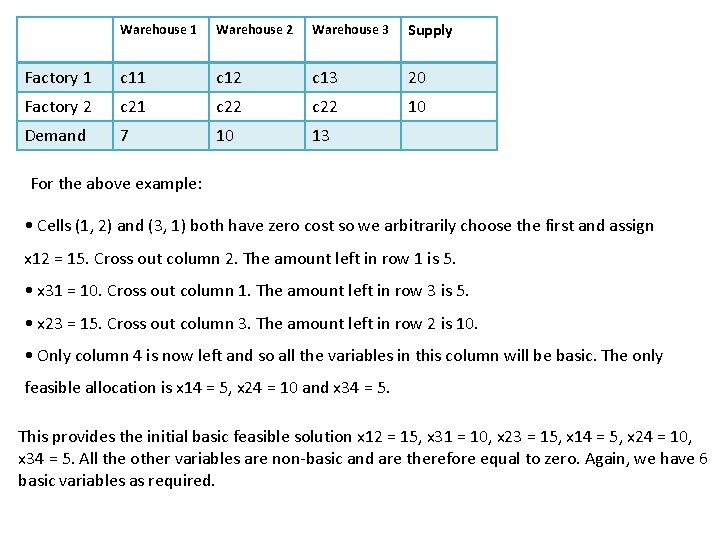
Warehouse 1 Warehouse 2 Warehouse 3 Supply Factory 1 c 12 c 13 20 Factory 2 c 21 c 22 10 Demand 7 10 13 For the above example: • Cells (1, 2) and (3, 1) both have zero cost so we arbitrarily choose the first and assign x 12 = 15. Cross out column 2. The amount left in row 1 is 5. • x 31 = 10. Cross out column 1. The amount left in row 3 is 5. • x 23 = 15. Cross out column 3. The amount left in row 2 is 10. • Only column 4 is now left and so all the variables in this column will be basic. The only feasible allocation is x 14 = 5, x 24 = 10 and x 34 = 5. This provides the initial basic feasible solution x 12 = 15, x 31 = 10, x 23 = 15, x 14 = 5, x 24 = 10, x 34 = 5. All the other variables are non-basic and are therefore equal to zero. Again, we have 6 basic variables as required.

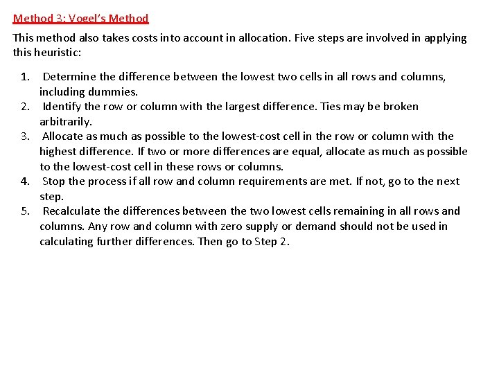
Method 3: Vogel’s Method This method also takes costs into account in allocation. Five steps are involved in applying this heuristic: 1. Determine the difference between the lowest two cells in all rows and columns, including dummies. 2. Identify the row or column with the largest difference. Ties may be broken arbitrarily. 3. Allocate as much as possible to the lowest-cost cell in the row or column with the highest difference. If two or more differences are equal, allocate as much as possible to the lowest-cost cell in these rows or columns. 4. Stop the process if all row and column requirements are met. If not, go to the next step. 5. Recalculate the differences between the two lowest cells remaining in all rows and columns. Any row and column with zero supply or demand should not be used in calculating further differences. Then go to Step 2.

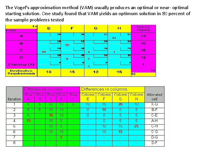
The Vogel's approximation method (VAM) usually produces an optimal or near- optimal starting solution. One study found that VAM yields an optimum solution in 80 percent of the sample problems tested

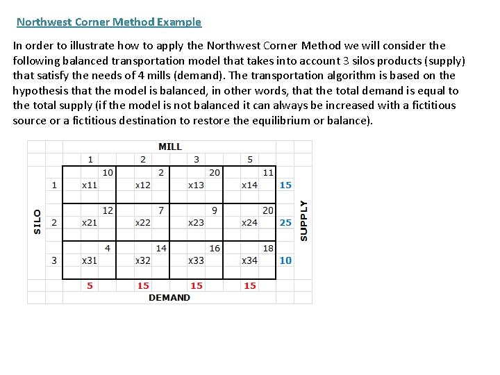
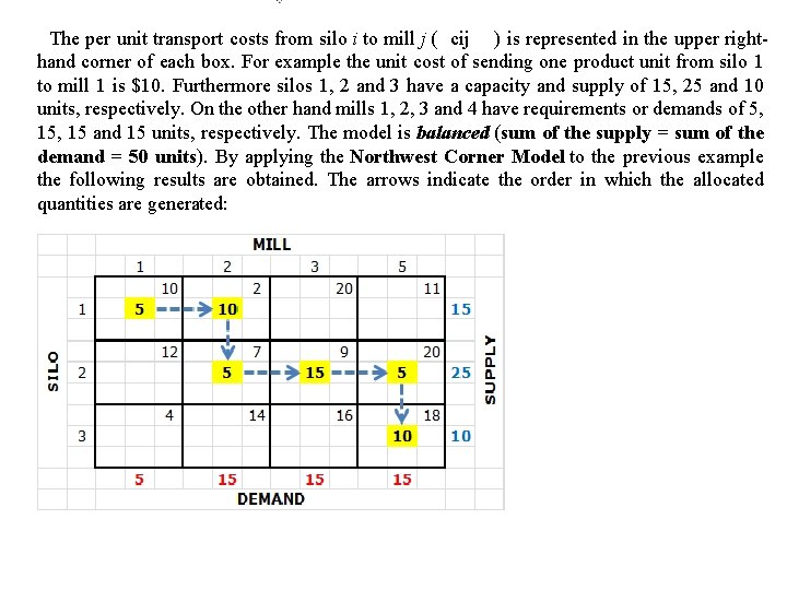
Northwest Corner Method Example In order to illustrate how to apply the Northwest Corner Method we will consider the following balanced transportation model that takes into account 3 silos products (supply) that satisfy the needs of 4 mills (demand). The transportation algorithm is based on the hypothesis that the model is balanced, in other words, that the total demand is equal to the total supply (if the model is not balanced it can always be increased with a fictitious source or a fictitious destination to restore the equilibrium or balance).

The per unit transport costs from silo i to mill j ( cij ) is represented in the upper righthand corner of each box. For example the unit cost of sending one product unit from silo 1 to mill 1 is $10. Furthermore silos 1, 2 and 3 have a capacity and supply of 15, 25 and 10 units, respectively. On the other hand mills 1, 2, 3 and 4 have requirements or demands of 5, 15, 15 and 15 units, respectively. The model is balanced (sum of the supply = sum of the demand = 50 units). By applying the Northwest Corner Model to the previous example the following results are obtained. The arrows indicate the order in which the allocated quantities are generated:

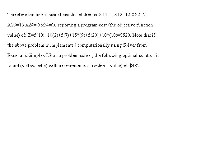
Therefore the initial basic feasible solution is: X 11=5 X 12=12 X 22=5 X 23=15 X 24= 5 x 34=10 reporting a program cost (the objective function value) of: Z=5(10)+10(2)+5(7)+15*(9)+5(20)+10*(18)=$520. Note that if the above problem is implemented computationally using Solver from Excel and Simplex LP as a problem solver, the following optimal solution is found (yellow cells) with a minimum cost (optimal value) of $435.

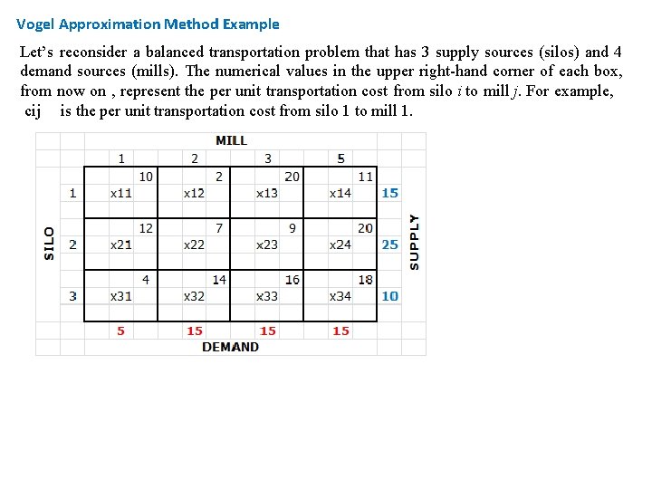
Vogel Approximation Method Example Let’s reconsider a balanced transportation problem that has 3 supply sources (silos) and 4 demand sources (mills). The numerical values in the upper right-hand corner of each box, from now on , represent the per unit transportation cost from silo i to mill j. For example, cij is the per unit transportation cost from silo 1 to mill 1.

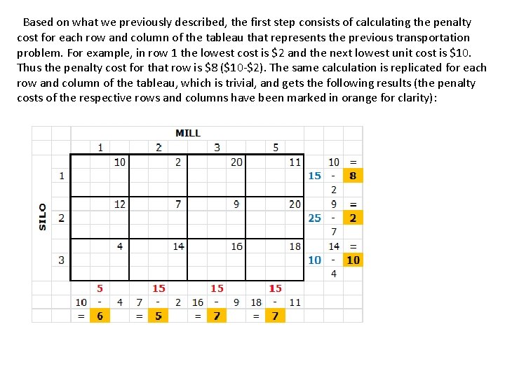
Based on what we previously described, the first step consists of calculating the penalty cost for each row and column of the tableau that represents the previous transportation problem. For example, in row 1 the lowest cost is $2 and the next lowest unit cost is $10. Thus the penalty cost for that row is $8 ($10 -$2). The same calculation is replicated for each row and column of the tableau, which is trivial, and gets the following results (the penalty costs of the respective rows and columns have been marked in orange for clarity):