Earthquake Design Using 1997 Uniform Building Code Dr

Earthquake Design Using 1997 Uniform Building Code Dr. Hathairat Maneetes Department of Rural Roads

The UBC was introduced in the 1927… • From the early 80’s, the earthquake design provisions in UBC changed rapidly and substantially in response to the lessons learned from several major earthquakes (e. g. 1971 San Fernando earthquake and 1994 Northridge earthquake) Soft story Spiral ties 1971 San Fernando earthquake Normal ties Another example of soft story Confinement effects

1997 UBC has several important modifications following the 1994 Northridge earthquake

Some of the major changes include • Strength-based (compared with allowable stress approach for the previous versions) • Removal of pre-qualified steel connection details • Requirements to consider liquefaction • Addition of near-fault factor to base shear formulation • Deformation compatibility requirements • Redundancy requirements • Stricter detailing for non-participating elements • Aligned with NEHRP’s provisions for smooth transition into International Building Code (IBC) in 2000

Three model buildings codes for seismic design in the United States. Three model building codes in US: – BOCA National Building Code (NBC) by BOCA – Uniform Building Code (UBC) by ICBO – Standard Building Code (SBC) by SBCCI NEHRP Materials code accompanying IBC SEAOC ASCE 7 BOCA NBC

There are three methods to estimate inertia or earthquake forces. Resultant (inertia) earthquake force distribution • Response (time) history method – Linear (elastic) or nonlinear (inelastic) – Apply acceleration history directly to base of numerical model of structure • Response spectrum method Ground acceleration Earthquake acceleration time – Linear (elastic) approach to calculate the modal (peak values) responses – Modal responses combined (using SRSS or CQC) to give design values • Equivalent static-force method – Linear approach (assume response dominated by 1 st mode response) Complexity – Nonlinear approach used for rehabilitation (“Push-over” analysis)

Typical response spectrum of a particular ground motion. Peak response acceleration, ar, peak Idealized for design purposes Actual Short to medium period Long Period (T) M K a Ground acceleration time Period

The equivalent static force procedure is a simplification of the dynamic response spectrum method. Consider more than one mode to get realistic results Response Spectrum Method T 6 T 5 T 4 T 3 T 2 T 1 Building model Equivalent Static force Method Multiple (e. g. six) degrees of freedom Decoupled SDOF Consider only the fundamental (1 st) mode to simply analysis T 1

UBC-97 is specific about which analysis method may or must be used. Static Lateral-force Procedure limitations: • • • All structures (regular or irregular) in Seismic Zone 1 or in Zone 2 with occupancy category 4 or 5. Regular structures using one of the structural systems listed in Table 16 -N if they are under 240 feet (7, 315. 2 cm) in height. Irregular structures not more than 5 stories or 65 feet (1, 981. 2 cm) in height. Seismic Zones Regular structure Irregular structure 1 2 A and 2 B (with occupancy category 4 or 5) 3, 4 < 240 feet < 5 stories or 65 feet

If these conditions are not satisfied, the structure shall be designed using dynamic method. • Structures with a flexible upper portion supported on a rigid lower portion if all of the following conditions are met: – When both portions are considered separately, they can both be classified as regular. – The average story stiffness of the lower portion is at least ten times the average story stiffness of the upper portion. – The period of the whole structure is no more than 1. 1 times the period of the upper portion considered as a separate structure fixed at the base. So how do we define building irregularities with respect to earthquake design?

There are two types of irregularities, on plan or along the building height. Vertical Irregularities Kx < 0. 7 Kx+1 or Kx < 0. 8 (Kx+1 + Kx+2 + Kx+3)/3 Where K is the story lateral stiffness x+3 x+2 x+1 x UBC-97 Table 16 -L Stiffness irregularity – soft story

There are two types of irregularities, on plan or along the building height. Vertical Irregularities Wx+1 > 1. 5 Wx or Wx+1 > 1. 5 Wx+2 Where W is the story effective weight (or mass) x+2 x+1 x UBC-97 Table 16 -L Weight (mass) irregularity

There are two types of irregularities, on plan or along the building height. Vertical Irregularities b 1 > Where bi: Horizontal 1. 3 b 2 dimension of lateral force -resisting system at story b 2 i Lateral force resisting elements b 1 UBC-97 Table 16 -L Vertical geometric irregularity

There are two types of irregularities, on plan or along the building height. Vertical Irregularities l 2: offset l 2 > l 1 l 2 l 1: length of lateral-load resisting elements l 1 UBC-97 Table 16 -L In-plane discontinuity in vertical lateral-force resisting element

There are two types of irregularities, on plan or along the building height. Vertical Irregularities Sx+1/Sx < 0. 8 Where S: Total strength of lateral force resisting elements x+1 x UBC-97 Table 16 -L Discontinuity in capacity – weak story

There are two types of irregularities, on plan or along the building height. Plan Irregularities UBC-97 Table 16 -M Torsional irregularity – to be considered when diaphragms are not flexible

There are two types of irregularities, on plan or Deformation along the building height. incompatibility Plan Irregularities Stiffer; less deformation Less stiff; more deformation leading to stress concentration Stress concentrations Re-entrant corners UBC-97 Table 16 -M

There are two types of irregularities, on plan or along the building height. Plan Irregularities Aopening > 0. 5 Agross Open Aopening Diaphragm discontinuity UBC-97 Table 16 -M

There are two types of irregularities, on plan or along the building height. Plan Irregularities Vertical lateral force resisting elements offset out-of-plane Out-of-plane offsets UBC-97 Table 16 -M

There are two types of irregularities, on plan or along the building height. Plan Irregularities These lateral force resisting elements are not parallel to major axes These lateral force resisting elements are not parallel and symmetric to major axes Nonparallel systems UBC-97 Table 16 -M

The UBC-97 governing equations are … Spectral Acceleration Estimation of Total Base Shear 2. 5 Ca Equation 30 -4 But need not be greater than Equation 30 -5 Ca But need to be at least Equation 30 -6 T 0 Ts Period (T) UBC-97 Design Spectra Equation 30 -7 (for Seismic zone 4)

Inertial forces is developed from Newton’s Second Law. Damping Lumped mass (M) ar = a ar = f(M, K, a, c) ar = a F = M ar F = M. a Flexible with stiffness K Infinitely rigid a Rigid box of mass M fixed to the ground a Ground acceleration RIGID BODIES a time NON-RIGID BODY

UBC-97 has broadly zoned US territories into six seismic zones. Seismic Zones 1 2 A 2 B UBC-97 Figure 16 -2: Seismic Zone Map of the United States 3 4 Increasing seismic risk 0

Each seismic zone is assigned a factor that corresponds to the maximum ground acceleration. Seismic Zone Factor Z 0 0 1 0. 075 2 A 0. 15 2 B 0. 2 3 0. 3 4 0. 4 UBC-97 Table 16 -I

The “effective” ground acceleration imparted to the structure is affected by the soil conditions. a = ag a a UBC-97 Table 16 -J Reference soil type ag Ground acceleration based on SB soil profile (i. e. rock). Default soil profile ag Other soil profiles tend to amplify the ground acceleration impart to the structure base a < ag (Hard rock, rock) a > ag (All other soil profiles)

Seismic coefficients represent the seismicity of the region and the characteristics of the soil. Seismic Coefficient Cv Seismic Coefficient Ca ag UBC-97 Table 16 -Q a “Short” to “medium” period UBC-97 Table 16 -R “Long” period

Response Modification Factor to account for nonlinear building response. • Need to consider the inherent ability of the structure to reduce the earthquake forces through overstrength, ductility and damping. • A response reduction factor or R-factor is introduced to account for the beneficial effects of nonlinear building behavior. • R-value greater than 1, inelastic response is assumed and earthquake forces is reduced. Base Shear Elastic response V Reduction in earthquake forces arising from nonlinear building response V/R “Actual” Inelastic response Higher ductility s M = (0. 7 R) s Displacement

R-value is a convenient method to describe the nonlinear response of the structural system. Total Base Shear V V/R 1 V/R 2 V/R 3 System 1 System 2 Increase in inelastic response System 3 R 3 > R 2 > R 3 Displacement

UBC-97 categories 7 basic structural systems with R-values varying from 2. 2 to 8. 5 • These are maximum values for each structural system type; lower value can be used if required. • Great care must be exercised in selecting the Rvalue! UBC-97 Table 16 -N

What are the common structural systems? Lateral Gravity Bearing wall • • • Supports all gravity and lateral loads Lack redundancy R-value varies from 2. 8 to 5. 5 Building frame • • Frame carries gravity (i. e. gravity frame Shear walls or braced frames carry lateral load Need to consider deformation compatibility R-value varies from 5. 5 to 7. 0 Dual system Moment-resisting frame • • • Specially detailed frame to support both gravity and lateral loads High level of ductility and redundancy R-value varies from 3. 5 to 8. 5 • • Similar to building frame system except the gravity frame also provide secondary lateral force resistance. R-value varies from 4. 2 to 8. 5

Examples of structural systems Building frames Column Beam Concentric braced frames (CBF) Moment frame Steel eccentric braced frame (EBF) Special truss moment frame Example of moment resisting connection Example of simple shear connection

For essential or hazardous buildings, the margin of safety in seismic design needs to be higher • The importance factor is used to increase the earthquake force • Depends on the occupancy category. • In UBC-97, I is 1. 25 for essential facilities and hazards facilities; no enhancement for other facilities. UBC-97 Table 16 -K

UBC-97 Load Combinations Strength level U = 1. 2 D + f 1 L + 1. 0 E U = 0. 9 D + 1. 0 E where E = Eh + Ev where Ev = 0. 5 Ca. ID Vertical component f 1 = 1. 0 for public assembly LL>100 psf(4. 9 k. N/m 2) = 1. 0 for garage LL = 0. 5 for other LL Working stress level F = D + (W or E/1. 4) F = 0. 9 D + (E/1. 4) F = D + 0. 75 [L + (Lr or S) + (W or E/1. 4)] Eh OR F = 4/3[D + L + (W or E/1. 4)] F = 4/3[D + L + (E/1. 4)] 1. 2 D + 0. 5 L + Ev

Numerical Example – Static lateral-force procedure Non-bearing • Determine the design seismic forces for the threestory reinforced concrete shear wall shown using UBC-97 static lateral-force procedure. The building is located in Southeastern California on rock with a shear wave velocity of 3, 000 ft/sec. The story dead loads are 2, 200 kips, 2, 000 kips and 1, 700 kips for the 1 st, 2 nd and roof level, respectively. The shear walls do not carry significant vertical loads. (Adapted from Naeim (2001)) IMPORTANT: Always check the applicability of the method • Building of regular construction • No plan or height irregularity • Total height = 35 feet < 240 feet UBC-97 static lateral-force method is applicable. shear wall 11 ft 13 ft Building is assumed to be located here UBC-97 Figure 16 -2: Seismic Zone Map of the United States

Numerical Example – Static lateral-force procedure • • • Seismic Importance Factor, I = 1. 0 (Assumed non-essential facility) Location is in Seismic Zone 3 Seismic Zone Factor, Z = 0. 3 Shear velocity = 3, 000 ft/sec. Soil Profile Type is SB i. e. , rock UBC-97 Table 16 Seismic -I Seismic Zone Factor Z 0 0 1 0. 075 2 A 0. 15 2 B 0. 2 3 0. 3 4 0. 4 UBC-97 Table 16 -J • Note corrections Seismic Coefficients: CV = 0. 3, Ca = 0. 3 UBC-97 Table 16 -Q UBC-97 Table 16 -R

Numerical Example – Static lateral-force procedure Response modification factor: • Non-load bearing shear wall, recommended highest R-value is 5. 5 • Height limit is 240 ft > 35 ft (OK) Note corrections UBC-97 Table 16 -N

Numerical Example – Static lateral-force procedure V (kips) Estimation of Total Base Shear But need not be greater than 1, 109. 7 804. 5 194. 7 But need to be at least design base shear = 804. 5 kips 0. 29 Period (sec)

Numerical Example – Static lateral-force procedure Vertical Distribution of the Earthquake Forces. Level x Story height hx (ft) Story weight wx (kips) Wxhx x 103 (kips. ft) Seismic force at each level Fx (kips) Story shear Vx (kips) Story overturning moment Mx (kips. ft) 3 35 1, 700 59. 5 351. 7 3, 869 2 24 2, 000 48. 0 283. 7 635. 4 10, 858 1 13 2, 200 28. 6 169. 1 804. 5 21, 317 Σ 5, 900 136. 1 804. 5 351. 7 kips Level 3 Use load combination! 283. 7 kips Level 2 U = 1. 2 D + 0. 5 L + 1. 0 E 169. 1 kips Level 1 U = 0. 9 D + 1. 0 E

Numerical Example – Static lateral-force procedure Determine story drift limits Maximum inelastic response displacement: M = 0. 7 R s Rearranging, we have s = M/0. 7 R Where M < 0. 025 h for T < 0. 7 sec (UBC-97, Section 1630. 10) 1 st story: s < (0. 025)(13)/0. 7(5. 5) = 1. 01 in Other stories: s < (0. 025)(11)/0. 7(5. 5) = 0. 858 in

Other important considerations • Orthogonal effects : 100% in one direction + 30% in the orthogonal effects (UBC-97 Section 1633. 1) • Multiple lateral force resisting systems; requirements of more restrictive one governs (UBC-97 Section 1633. 2. 2) • Seismic design connections must be clearly detailed in drawings (UBC-97 Section 1633. 2. 3) • Deformation compatibility (UBC-97 Section 1633. 2. 4) • Familiarity with accompanying material codes , etc.

Time History Analysis. . . Oakland, CA

The natural frequencies fell within the dominating frequency range of the ground motions. GILROY EL CENTRO HOLLISTER

The 3 OR 7 pairs of recorded ground motions were scaled to match the design spectrum. SRSS of GILROY (N-S and E-W) x scale factor 1 0. 2 T 1. 5 T PGA = 0. 367 g SRSS of EL CENTRO (N-S and E-W) x scale factor 2 Average response spectrum PGA = 0. 371 g 1. 4 x Design Spectrum SRSS of HOLLISTER (N-S and E-W) x scale factor 3 PGA = 0. 177 g If 3 analyses performed, use the maximum response. If 7 analyses performed, use the average response.

An Innovative Design – Structural Control

What’s an innovative design? ? ? Conventional design – – – ductility-based approach nonlinear behavior of the structure Some damage may occur Energy-based design – – – ‘protective approach’ ‘structural control’ classified into 3 groups: passive, active and semiactive, hybrid controls

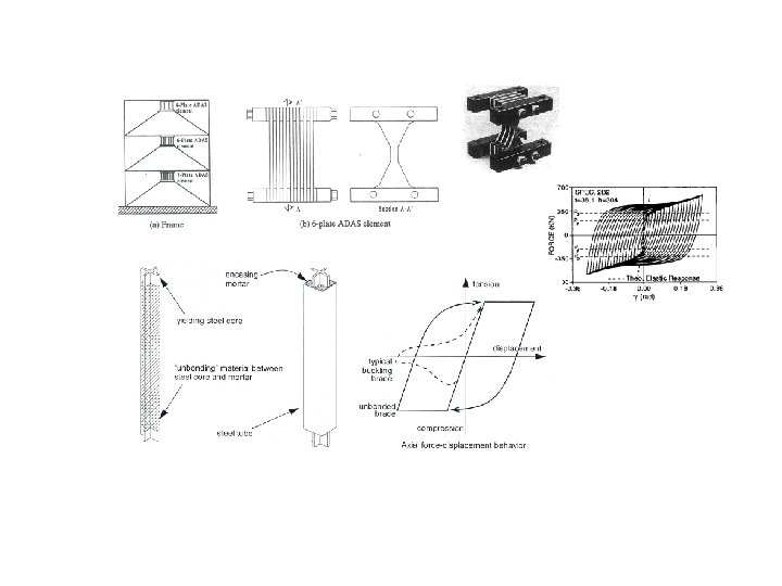
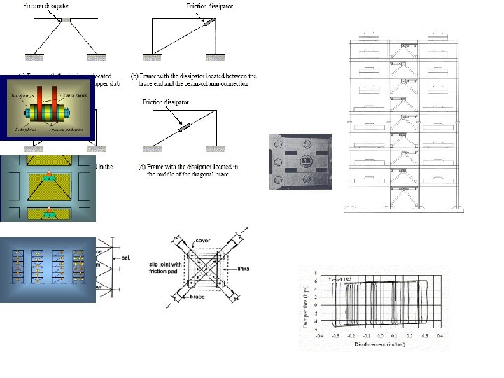
INTRODUCTORY - Passive Control • Incorporating passive devices to control the structural motion and to modify its dynamic parameters (stiffness and damping). Seismic (base) isolation Passive EDS Mass damper

INTRODUCTORY - Passive Control Source-Sink Analogies [Popov et al. , 1993]

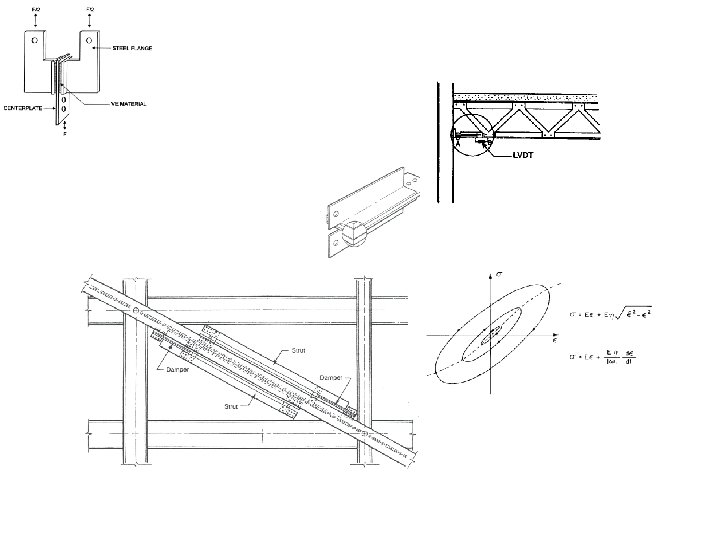
Viscous Fluid Damper

How to choose the appropriate system for your building? ? ? http: //www. oiles. co. jp/en/menshin/building/index. html

INTRODUCTORY - Active Control • Control motion of structure through some external energy source. Schematic Details [Chaidez, 2003] Analogy with Human Body (Servio Model)

INTRODUCTORY – Hybrid Systems A series or parallel combination of an active (or semiactive) system with a passive system. Active Control with Base Isolation System [Chaidez, 2003; Iemura, 1994]

Thank you for your attention! Any Questions ? ? ?