Earth Remote Sensing with Satellite Navigation Signals IEEC

Earth Remote Sensing with Satellite Navigation Signals IEEC Current projects A. Rius IEEC, September 2004

Earth Science and Technology Department § Antonio Rius § Pedro Elosegui § Oleguer Nogues § Serni Ribó § Josep Sanz § Txepo Torrobella Badía § Myrthe Beekhuis § Santi Oliveras § Benji Garzon Consultores § Josep Maria Aparicio, Inst. Met Canada § Estel Cardellach, Cf. A. Enero 2005 de la Cierva

Occultations Beam of rays Refractivity gradient Transmitter Receiver

Reflections Receiver (space, aircraft, ground. . . ) Transmitter (GPS (DOD) or Radio Source (GOD) or RADAR) Planet, satellite,

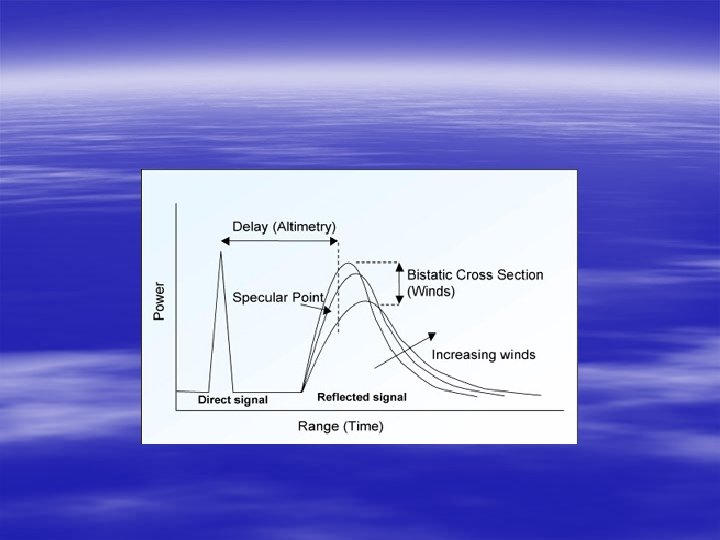
Direct signal Reflected signal Receiver direct Specular point el 2* h* sin (el ) 2*h Receiver reflected Doppler Delay mapping

Scattering (nadir case)

Scattering (oblique case)

Geodetic Techniques Ø Space Geodetic and related Techniques at microwave frequencies: Ø Very Long Baseline Interferometry Ø Global Positioning System Ø Other GNSS Ø Radar altimeters Ø The observables are differences in the arrival epochs of microwave signals. These differences are affected by the atmospheric refractivity or the surface scattering properties. 8

Global Navigation Satellite Systems § Global Positioning System (GPS/USA) [24] § GLObal’naya Navigatsionnaya Sputnikova Sistema (GLONASS/ Russia) [24] § future GALILEO? (EU) [30] § Communication Satellites: Inmarsat [4], Artemis [1] Potentially, 50 -80 satellites freely transmitting L-band coded signal

Resources Ø 24 operational satellites at an altitude of 20, 000 km. Ø Transmit ranging data (1. 2 and 1. 6 GHz) to ground -based receivers. Ø The GPS system measures time delays between the transmission and reception of the electromagnetic signals. Ø These delays contain information on the distance between satellites and receivers: geometric delay. Ø Delays are also affected by the presence of matter along the path: atmospheric delay (ionosphere and troposphere) gravitational delay. Ø the atmosphere affects the signal propagation Ø extra delay (slowing effect) Ø curved path (bending effect) Ø GPS Meteorology Ø The sea surface is a good conductor at L Band. The signal could be reflected on the sea surface or ice, snow, . . Ø GPS Oceanography 10

Global Navigation Satellite Systems: GPS signal

Global Navigation Satellite Systems: GPS signal § 2 carriers, common to all transmitters: L 1=1. 575 GHz L 2=1. 228 GHz § Code Division Multiple Access: phase modulation by orthogonal Pseudo. Random Noise, characteristic of each transmitter. § Current PRN-Codes: – C/A coarse, 300 m, P=1 ms (L 1) – P precise, 30 m, P=1 week, encrypted § Navigation message: 50 bps

IGS Network 13

Objectives Ø Space Geodetic Techniques objectives ØTo provide coordinates to points (position and time) in well defined reference frames ØThe receivers are placed in moving platforms : Ø Earth crust (cm/year) Ø LEOs Ø Airplanes Ø Sea buoys Ø Balloons (wind speed radiosondes) ØThe signal path could be: Ø “deterministic” or “random” Ø Direct or after reflection

Measurements Ø Space Geodetic Techniques: Measurements Ø Phase and group Delays experienced by EM signals from transmitter to receiver antennas. Ø The precision of the phase measurements is below 1 mm after 1 second of integration. Ø The accuracy is in the order of 1 meter for the group delays (pseudoranges) Ø Delays depends on Ø The physical structure of the antennas Ø The geometry and dynamics of the antennas Ø The path followed by the signal Ø The EM properties of the medium traversing the signal Ø Instrumental errors in the receivers and in the transmitters

Analysis Ø Space Geodetic Techniques: Analysis Ø The measurements are analyzed with a (simplified) model, defined trough a set of stochastic processes Ø Receiver coordinates (including geophysical phenomena) Ø Transmitter coordinates (including phenomena perturbing the orbits) Ø Ionosphere and troposphere refractivity Ø Antenna phase patterns Ø Instrumental biases Ø Because the correlations among the stochastic processes it is not possible to solve for everything. Ø The selection of the processes to estimate depends on the application.

Results Ø Space Geodetic Techniques: Results (typical) Ø Typical precisions of the estimations are: Ø 5 mm for the receiver coordinates Ø 5 cm for the transmitter coordinates Ø 1 cm for the zenith tropospheric delay ØBelow these quantitities the system is controled by coloured noise

Ø One man’s trash is another man’s treasure Ø One man’s signal is another man’s noise High accuracy geodetic systems ZTD, WZD IWV Multipath Scattering Nuisance parameters NWP models Ocean models model

The tropospheric delay Observed delay = geometrical delay + ionospheric delay + tropospheric delay + instrumental delay ØThe geometrical delay can be computed from the positions of the transmitter and the receiver. The position can be modeled with geophysical information which accounts for Earth tides, ocean loading, etc. ØThe ionospheric delay depends on the frequency and can be removed using two different frequencies. ØInstrumental effects are essentially time independent (scale of minutes). Observed delay – corrections = tropospheric delay But, notice that with this definition the tropospheric delay are “correlated measures”

Ø WV is a small fraction of atmospheric gases (fractional volume 0 - 4 %). Ø Distribution and content are critical for the description of the state and evolution of the atmosphere. Ø Highly variable in time and space and correlates poorly with surface humidity measurements. Ø Lack of precise and continuous WV data is one of the major error sources in short-term forecasts of precipitation (Kuo et al. 1993, 1996).

Ø Current observational techniques: l radiosondes (expensive, poor temporal resolution, poor spatial coverage) l ground-based and space-based WVR (poor spatial coverage or poor temporal resolution, expensive). Ø A new observational technique (Bevis et al. 1992): GPS system precise and continuous estimates of WV

Ø The tropospheric delay of the GPS signal is the integral of the refractivity N along the ray path. Ø Neglecting liquid water contribution and ionospheric effects (Smith and Weintraub 1953), Ø Ø Ø Slant Troposheric delay Zenith Tropospheric Delay (ZTD) ZTD is estimated with a formal error of 5 mm (Businger et al. 1996) at around 10 -min interval.

Zenith Hydrostatic delay (ZHD) Ø typical value of 2300 mm at sea level. Ø accurately modeled if measurements of surface pressure (barometer or a NWP model) are available (Saastamoinen 1972). Ø error of 0. 4 mb in Ps less than 1 mm error of ZHD

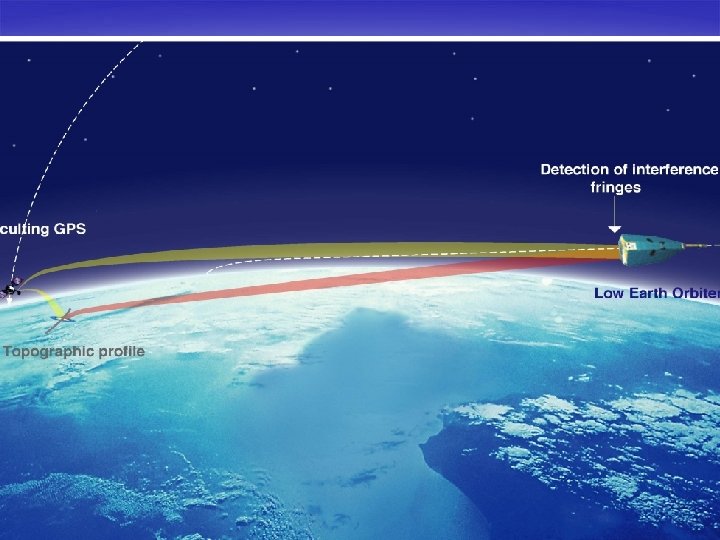
GPS Radio Occultation § The 24 GPS satellites are distributed roughly in six circular orbital planes at ~55 o inclination, 200 km altitude and ~12 hour periods. § Each GPS satellite continuously transmits signals at two L-band frequencies, L 1 at 1. 57542 GHz (~19 cm) and L 2 at 1. 227 GHz (~24. 4 cm). § A ray passing through the atmosphere is refracted due to the vertical gradient of density. GPS satellite Low Earth Orbiting (LEO) satellite

Future GPS Occultation Missions Metop is the European component of the joint Europe/US polar satellite system It will have a GPS receiver for occultations. METOP

Future GPS Occultation Missions COSMIC It is planned to be launched in spring 2005 1) Six spacecraft 2) GPS receiver

GPS Occultation Used to probe planetary atmospheres (1970 -. . . ) The bending of the radio path provides information on the vertical distribution of the refractivity The bending produces an additional (and measurable) doppler shift in the signal GPS made possible to apply the technique to the Earth. It provides vertical resolution better than 1 km. Earth Ionosphera Troposphera Occulting LEO

Occultations vs. Radio Sondes

Metop will use a GPS fiducial network. Metop will need to estimate orbits, satellite clocks, etc as in ground based GPS meteorology The GRAS Ground segment has resources useful for ground GPS meteorology Synergy

Usual approaches In general, a key ingredient is to use linear algorithms as much as possible §Robustness: Non-linear algorithms risk to be unstable, non convergent. . . §Speed: Processing time for linear algorithms is predictable, and in general small. §Accuracy: Allowing non linearity is

First approaches to occultation processing § Simple and fast algorithms exist: Doppler evaluation – Bending angles & impact parameters – Abel transform – § This solves the problem of extracting some quick solution § However: Not very accurate – Algorithmically weak against cycle slip –

Some reflections before proceeding § What is missing in the Abel approach? We are actually extracting the atmospheric structure from scratch at every profile – In early radiooccultations (Venus, Mars), this was necessary: the target was the climatic profile – But we are looking here for the meteorological info: i. e. the departure from the climatic profile – Hint:

Subtraction of known information § It is standard to subtract vacuumpropagated values of phase, Doppler, etc. § But we know enough about the Earth's atmosphere to be able to subtract

Climatic subtraction issues I § The climatic subtraction requires a raytracing (comparatively expensive and risky) However: § Unlike gridded ones, the climatic model tested (MSISE) is sufficiently well behaved for the raytracing to predictably converge and succeed § Not all samples need to be traced.

Climatic subtraction issues II § Atmospheric radius of curvature depends on the direction, and even changes during an occultation § Algorithms based on spherical symmetry are contaminated by this (not only by horizontal gradients!) § Most of the contamination from the ellipsoidal shape and variable curvature is removed with climatic raytracing

Zenith Wet delay (ZWD) Ø smaller value (0 -300 mm) Ø very difficult to model: highly variable in space and time. Ø associated with Precipitable Water (PW). Ø If surface pressure measurements are available, ZWD = ZTD - ZHD ~ 6. 6 PW Ø PW can be retrieved with a rms error of around 1 mm (Herring 1990, Rocken et al. 1997).

Motivation § GNSS: Global Navigation Satellite System – Compound by a large constellation of satellites, transmitting coded signals – Direct reception by the user (ground, aircraft, spacecraft) for positioning purposes.

Motivation: GNSS reflection concept § Main advantages of the GNSSr concept: – FREE SIGNALS, ALREADY EXIST – PASSIVE – MULTISTATIC Tropospheric delay Sea level, SWH, roughness/wind salinity, ice, oil. . .

§ 1956 : radiosources observed with sea interferometer § Radar astronomy (meteorites also!) § 1970: [Peterson et al. ] proved the sensitivity of bistatic radar at radiowaves from ground-based stations. § 1993: [Martín-Neira] proposes the PARIS concept: PAssive Reflectometry and Interferometry System. § 1998: studies of GPSr for altimetry and sea surface topography.

The PARIS concept

Modelling the GNSS reflected signal § Dielectric proprieties of the sea water: capacity to reflect Lband signals.

Modelling the GNSS reflected signal § Each point on the sea surface has certain capability to forward the incoming signal in the direction of the receiver: scattering coefficient s 0

Modelling the GNSS reflected signal § Mean Square Slope (mss) is the parameter accounting for the sea roughness, linked to the wind through different models (Elfouhaily, Apel, …)

Modelling the GNSS reflected signal

Modelling the GNSS reflected signal BUT: the signals reflected from different points on the sea surface have different relative delay.

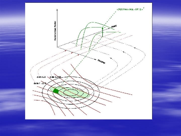
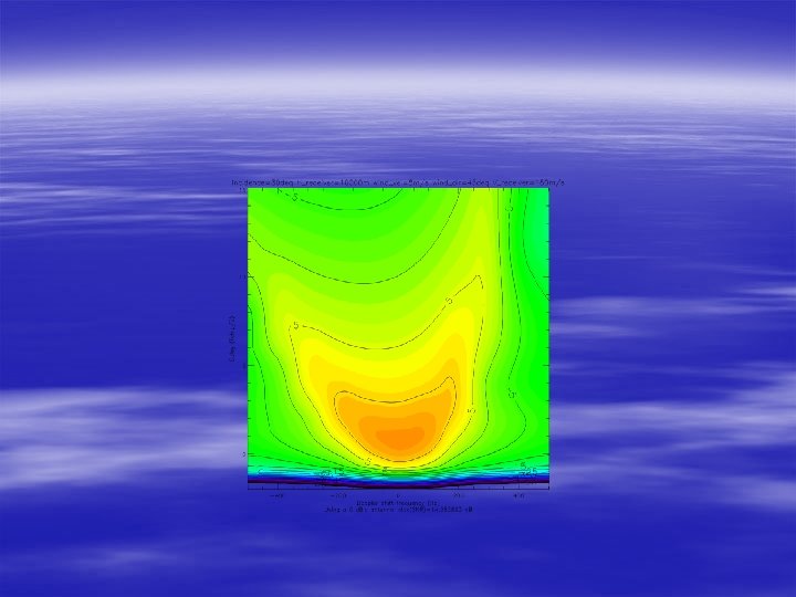
Modelling the GNSS reflected signal MOREOVER: the signals reflected from different points on the sea surface have different Doppler frequency offset. It is possible, thus, to MAP the illuminated area by correlating the signal with replicas of the code at different DELAY lags and DOPPLER frequencies.

Modelling the GNSS reflected signal § Hence, the squared correlation function for different delay-Doppler lags (waveform) contains information about the distribution of the reflected power along the sea surface

System Analysis QUESTION-1, SUMMARY: § Aircraft (10 km): wind vector retrieval better than [1 m/s, 15 deg] up to 17 m/s § LEO (350 km): wind speed retrieval better than 2 m/s up to 15 m/s. The direction can be inferred (<30 deg) using 100 chips of the waveform: – Low spatial resolution – instrumental drawbacks New inversion techniques

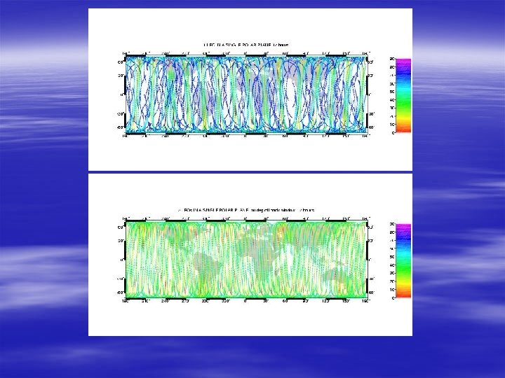
System Analysis QUESTION-2: coverage from space § Tool: specular locator [Aparicio et al. , 2000], given a GPS orbits file and the LEO/s parameters, it computes the location of the specular reflection points and informs about its geometry (elevation, receiver off nadir angle. . . ) § Cases: 1 LEO; 3 LEO-1 PLANE; 3 LEO-3 PLANES polar orbits, at 350 -400 km altitude.

System Analysis QUESTION-2, SUMMARY: § 1 LEO (350 -400 km): good coverage, near the User Requirements (UR). Global representation in 12 h. UR binning time: 72 h. § 3 LEOs-1 PLANE: UR binning time and Global representation: 12 h. § 3 LEOs-3 PLANES: UR binning time in 24 h. Global representation: 4 h. Multistatic character yields useful coverage

Experimental work § CASABLANCA – ESTEC/IEEC/Repsol collaboration. Validation of the delay-Doppler software pre-processor. 20. 5 MHz raw data § MEBEX – NASA/IEEC/ASI/INTA collaboration. Delaymap Hardware receiver on board a stratospheric balloon. 1 Hz Delaywaveforms.

Experimental work: CASABLANCA

Experimental work: MEditerranean Balloon EXperiment

Experiment overview:

Bistatic Altimetry:

Determination of relative delays for altimetry

Doppler mapping for scatterometry:

Processed data § The data is stored in a 3 D grid: – delay lag – frequency offset – time § Visualisation with vis 5 d

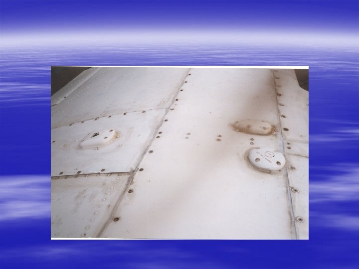
GPS antennas at sea

Reference station (to estimate tropospheric delays)

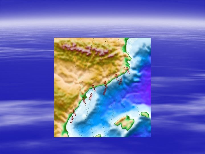
Mapping the sea surface using buoys equipped with GPS receivers The straight line is the T/P subtrack path At the points A, B, C, D, E, H, I the buoys collected data for one hour. At point O data was collected permanently to monitor systematic variations of the sea level

Comparison Topex/Poseidon vs GPS buoys The green crosses are GPS estimates at the points along the T/P track The blue points are T/P mean sea level values

Glistening surface

Filters in the radar equation

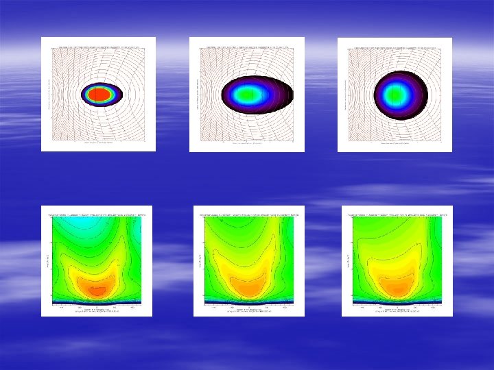
Delay-Doppler Mapping Each point in the sea surface could be clasified according to: a) Is inside the glistening surface? b) Its isodelay-isodoppler coordinates Note that there ambiguities The observable is the power detected as a function of the iso-delay and the iso-doppler coordinates

Comparison Topex/Poseidon vs GPS buoys The green crosses are GPS estimates at the points along the T/P track The blue points are T/P mean sea level values

GOLD-RTR The IEEC’s aircraft sensor based on the PARIS concept Authors: • Toni Rius (Project Manager) • Josep Sanz (Instrument Software Developer Engineer) • Josep Torrobella (Hardware Engineer) • Oleguer Nogués (System and Hardware Engineer) IEEC owns the copyright of this document which is supplied in confidence and which shall not be used for any purpose other than that of which it is supplied, and shall not in whole or in part be reproduced, copied, or communicated to any person without written permission from the owner.

General features (I) • GOLD-RTR stands for “GPS Open Loop Differential Real Time Receiver”. It’s purpose is to give the same products as the PARIS Aircraft Demonstrator (PAD): Functionality: computesin. Real-Timethe. PRNcodecomplexcorrelationfunctions around the peak (waveforms) for all the selected GPS visible satellites. Applications: The instrument can be used in both altimetry&scatterometry (PARIS), but also in occultation experiments.

General features (II) • The instrument is divided in two physical devices: a PC laptop running under LINUX and a rack with the custom instrumentation Laptop: 3 kg weight, Rack: 20 kg weight, 30 x 4 (cm), 30 W power (220 AC, 50 Hz) 35 x 45 x 55 (cm), 60 W power (220 AC, 50 Hz) both parts are linked via an UTP ethernet cable (RJ 45 connectors, cat. 5)

Instrument parts description (II) RACK BACK PANEL: Picture overview RF Connectors RJ 45 ethernet connector Power con. and switch Cooling fan holes

Instrument parts description (IV) RACK INSIDE contents: Graphical overview

Instrument parts description (V) RACK SP: Graphical overview

User’s instrument operation (VI) SOE file preparation software (snapshot)

User’s instrument operation (VII) Instrument control Software • It is a GUI that makes it easy to the FO actor to control the instrument, either to perform readiness tests or to upload a SOE file to perform an experiment. • When the GUI is started, a window appears (these are 2 examples of the same): Left: the GUI is not receiving flags information from the RACK Right: The GUI is receiving information from the RACK

User’s instrument operation (IX) Rediness Test Graphical Results