EART 20170 Computing Data Analysis Communication skills Lecturer

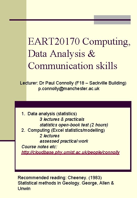
EART 20170 Computing, Data Analysis & Communication skills Lecturer: Dr Paul Connolly (F 18 – Sackville Building) p. connolly@manchester. ac. uk 1. Data analysis (statistics) 3 lectures & practicals statistics open-book test (2 hours) 2. Computing (Excel statistics/modelling) 2 lectures assessed practical work Course notes etc: http: //cloudbase. phy. umist. ac. uk/people/connolly Recommended reading: Cheeney. (1983) Statistical methods in Geology. George, Allen & Unwin

Lecture 1 KNOWLEDGE What do we know? Lecture 2 Lecture 3

Recap – first lecture n The four measurement scales: nominal, ordinal, interval and ratio. n There are two types of errors: random errors (precision) and systematic errors (accuracy). n Basic graphs: histograms, frequency polygons, bar charts, pie charts. n Gaussian statistics describe random errors. n The central limit theorem n Central values, dispersion, symmetry n Weighted mean. back

Recap – last lecture n Correlation between two variables n Classical linear regression n Reduced major axis regression n Propagation of errors back

Lecture 3 n Distribution of a continuous variable Normal distribution n Standardised normal distribution n Confidence limits n Students t distribution n n Statistical inference for two independent variables. Students t test n Hypothesis testing n back

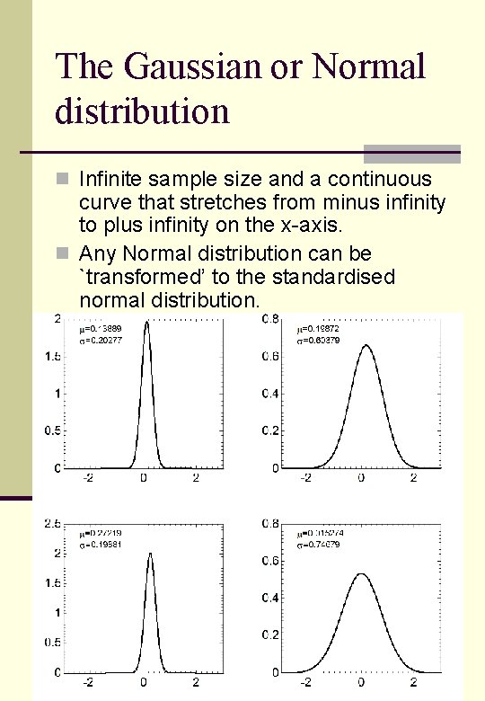
The Gaussian or Normal distribution n Infinite sample size and a continuous curve that stretches from minus infinity to plus infinity on the x-axis. n Any Normal distribution can be `transformed’ to the standardised normal distribution.

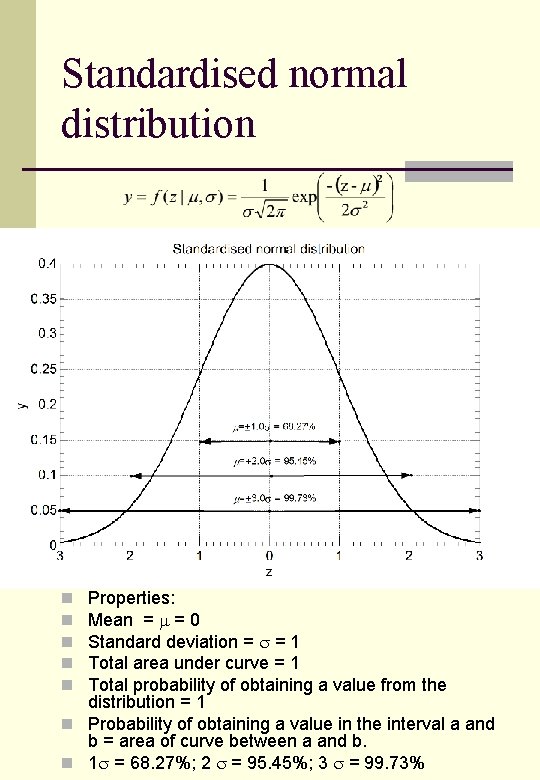
Standardised normal distribution Properties: Mean = = 0 Standard deviation = = 1 Total area under curve = 1 Total probability of obtaining a value from the distribution = 1 n Probability of obtaining a value in the interval a and b = area of curve between a and b. n 1 = 68. 27%; 2 = 95. 45%; 3 = 99. 73% n n n

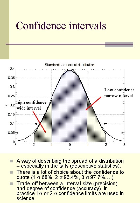
Confidence intervals Low confidence narrow interval high confidence wide interval n A way of describing the spread of a distribution – especially in the tails (descriptive statistics). n There is a lot of choice about the confidence to quote (1 68%, 2 95. 4%, 3 97. 7%…. ) n Trade-off between a interval size (precision) and degree of confidence (accuracy). In practice 1 or 2 confidence limits are used in science.

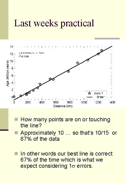
Last weeks practical n How many points are on or touching the line? n Approximately 10 … so that’s 10/15 or 67% of the data n In other words our best line is correct 67% of the time which is what we expect considering 1 errors.

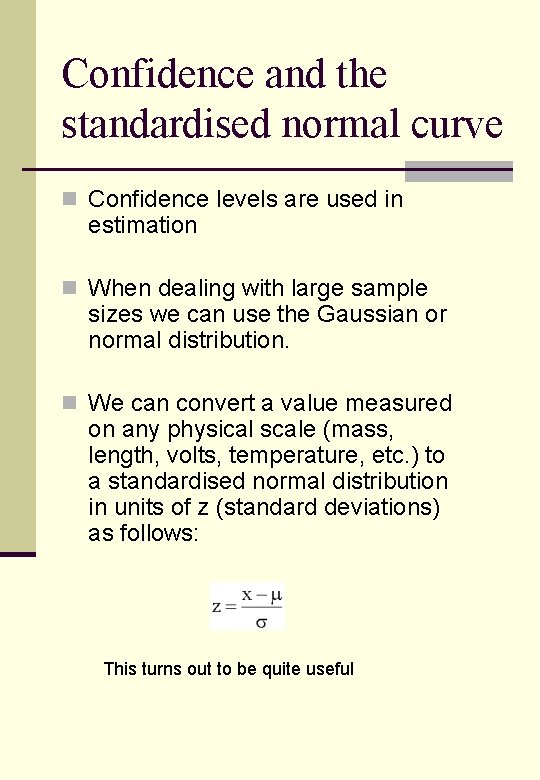
Confidence and the standardised normal curve n Confidence levels are used in estimation n When dealing with large sample sizes we can use the Gaussian or normal distribution. n We can convert a value measured on any physical scale (mass, length, volts, temperature, etc. ) to a standardised normal distribution in units of z (standard deviations) as follows: This turns out to be quite useful

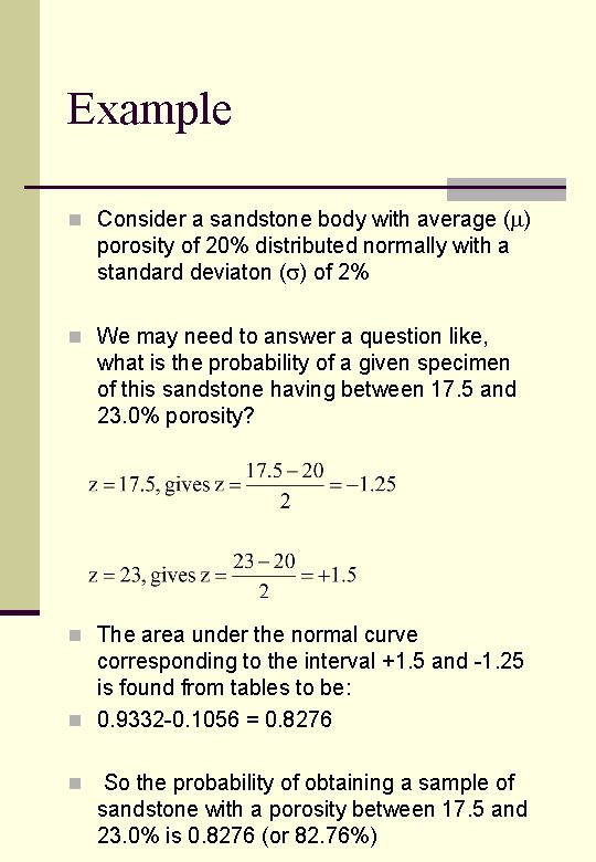
Example n Consider a sandstone body with average ( ) porosity of 20% distributed normally with a standard deviaton ( ) of 2% n We may need to answer a question like, what is the probability of a given specimen of this sandstone having between 17. 5 and 23. 0% porosity? n The area under the normal curve corresponding to the interval +1. 5 and -1. 25 is found from tables to be: n 0. 9332 -0. 1056 = 0. 8276 n So the probability of obtaining a sample of sandstone with a porosity between 17. 5 and 23. 0% is 0. 8276 (or 82. 76%)

Student t distribution n The t distributions were discovered by William S. Gosset in 1908. Gosset was a statistician employed by the Guinness brewing company which had stipulated that he not publish under his own name. He therefore wrote under the pen name ``Student. '' These distributions arise in the following situations.

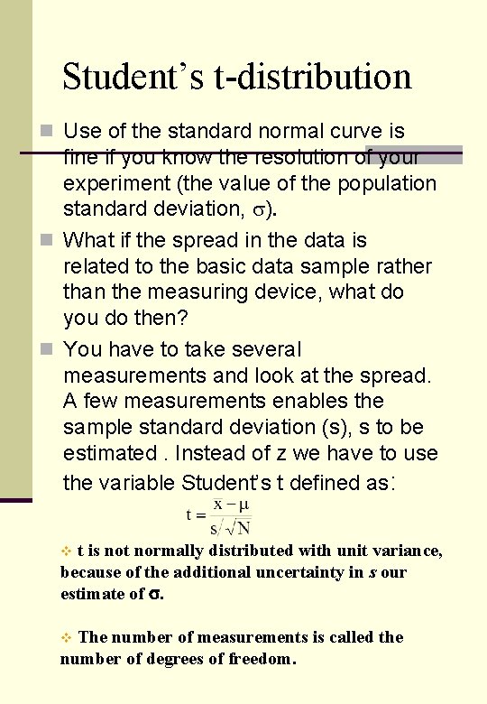
Student’s t-distribution n Use of the standard normal curve is fine if you know the resolution of your experiment (the value of the population standard deviation, ). n What if the spread in the data is related to the basic data sample rather than the measuring device, what do you do then? n You have to take several measurements and look at the spread. A few measurements enables the sample standard deviation (s), s to be estimated. Instead of z we have to use the variable Student’s t defined as: t is not normally distributed with unit variance, because of the additional uncertainty in s our estimate of s. v The number of measurements is called the number of degrees of freedom. v

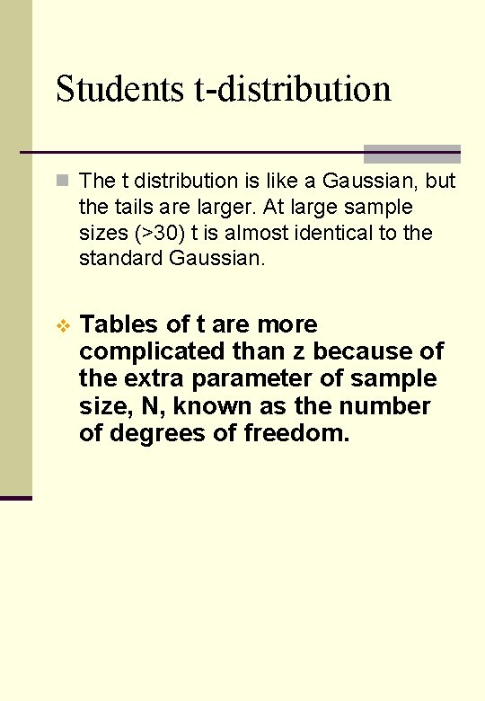
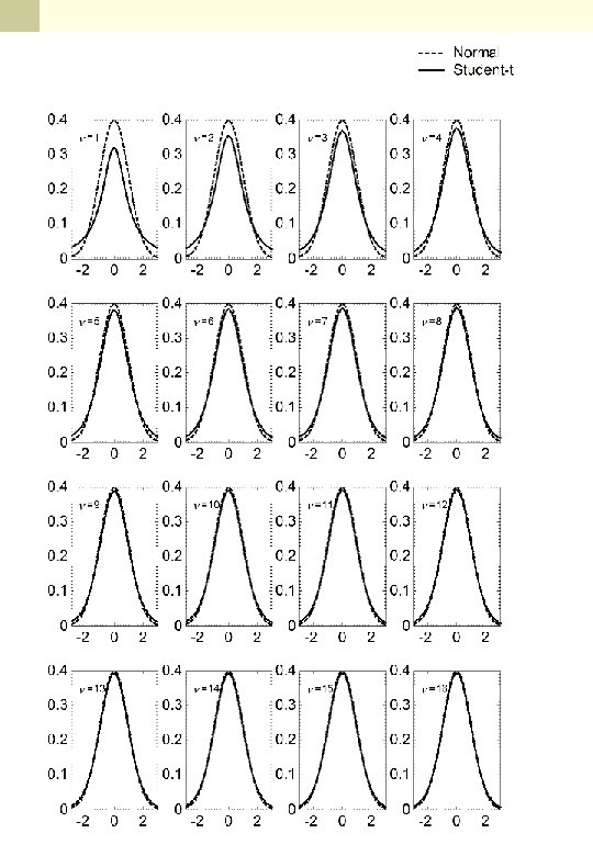
Students t-distribution n The t distribution is like a Gaussian, but the tails are larger. At large sample sizes (>30) t is almost identical to the standard Gaussian. v Tables of t are more complicated than z because of the extra parameter of sample size, N, known as the number of degrees of freedom.

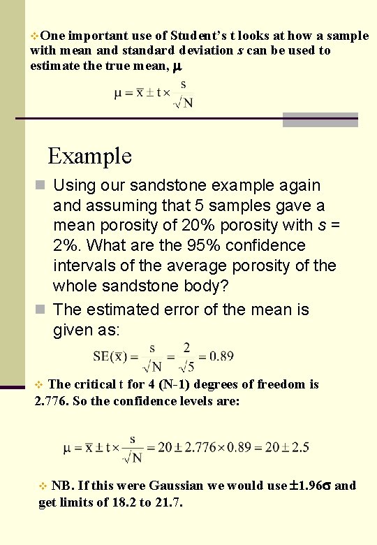
v. One important use of Student’s t looks at how a sample with mean and standard deviation s can be used to estimate the true mean, m Example n Using our sandstone example again and assuming that 5 samples gave a mean porosity of 20% porosity with s = 2%. What are the 95% confidence intervals of the average porosity of the whole sandstone body? n The estimated error of the mean is given as: The critical t for 4 (N-1) degrees of freedom is 2. 776. So the confidence levels are: v NB. If this were Gaussian we would use 1. 96 s and get limits of 18. 2 to 21. 7. v

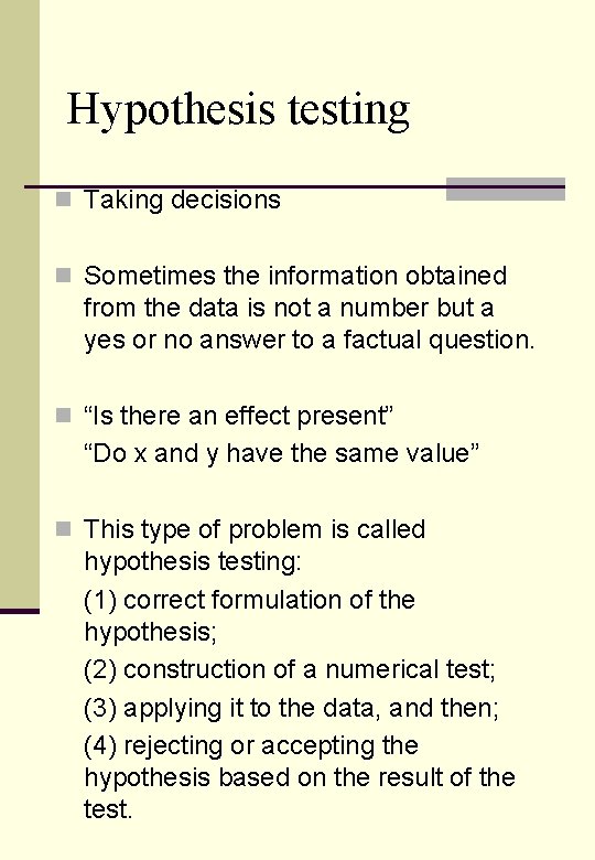
Hypothesis testing n Taking decisions n Sometimes the information obtained from the data is not a number but a yes or no answer to a factual question. n “Is there an effect present” “Do x and y have the same value” n This type of problem is called hypothesis testing: (1) correct formulation of the hypothesis; (2) construction of a numerical test; (3) applying it to the data, and then; (4) rejecting or accepting the hypothesis based on the result of the test.

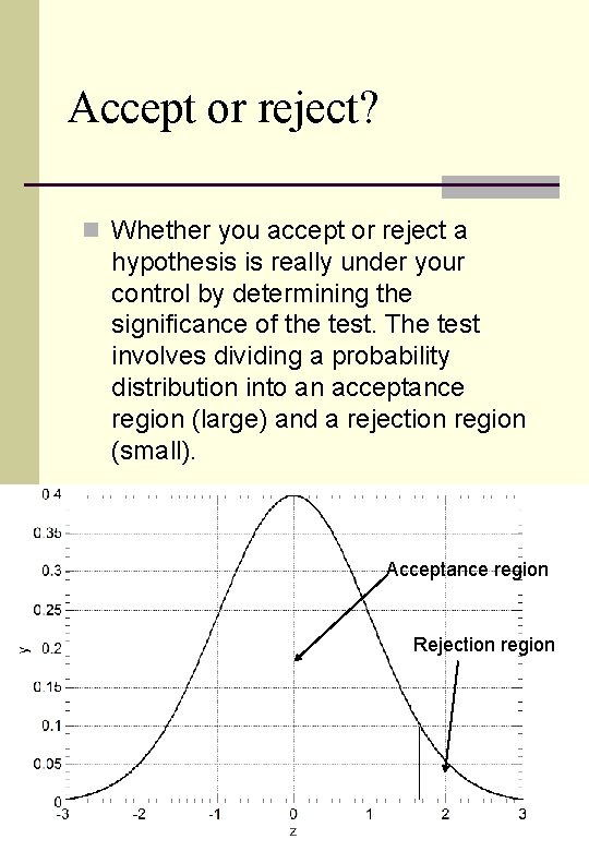
Accept or reject? n Whether you accept or reject a hypothesis is really under your control by determining the significance of the test. The test involves dividing a probability distribution into an acceptance region (large) and a rejection region (small). Acceptance region Rejection region

Significance n The significance of a test is called and is the rejection region of our probability distribution. For a good test should be small – 1% or 5%. n The hypothesis is usually the null effect (i. e. no difference, no effect), but the alternate hypothesis tends to be vague and unquantifiable (e. g. an effect exists but gives no clue as to why or how large). n Final point is to remember that there is a difference between one-tailed directional and two-tailed non-directional tests. “X is greater than Y” is a one-tailed test “X is different from Y” is a two-tailed test

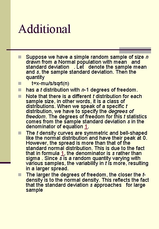
Additional n Suppose we have a simple random sample of size n n n n drawn from a Normal population with mean and standard deviation . Let denote the sample mean and s, the sample standard deviation. Then the quantity t=x-mu/s/sqrt(n) has a t distribution with n-1 degrees of freedom. Note that there is a different t distribution for each sample size, in other words, it is a class of distributions. When we speak of a specific t distribution, we have to specify the degrees of freedom. The degrees of freedom for this t statistics comes from the sample standard deviation s in the denominator of equation 1. The t density curves are symmetric and bell-shaped like the normal distribution and have their peak at 0. However, the spread is more than that of the standard normal distribution. This is due to the fact that in formula 1, the denominator is s rather than sigma. Since s is a random quantity varying with various samples, the variability in t is more, resulting in a larger spread. The larger the degrees of freedom, the closer the tdensity is to the normal density. This reflects the fact that the standard deviation s approaches for large sample

Hypothesis testing n A hypothesis test is a procedure for determining if an assertion about a characteristic of a population is reasonable. n For example, suppose that someone says that the average price of a gallon of regular unleaded gas in Massachusetts is $1. 15. How would you decide whether this statement is true? n You could try to find out what every gas station in the state was charging and how many gallons they were selling at that price. That approach might be definitive, but it could end up costing more than the information is worth. n A simpler approach is to find out the price of gas at a small number of randomly chosen stations around the state and compare the average price to $1. 15. n Of course, the average price you get will probably not be exactly $1. 15 due to variability in price from one station to the next. Suppose your average price was $1. 18. n Is this three cent difference a result of chance variability, or is the original assertion incorrect? A n hypothesis test can provide an answer.

Hypothesis test terminology n The null hypothesis is the original assertion. In this case the null hypothesis is that the average price of a gallon of gas is $1. 15. The notation is H 0: µ = 1. 15. n There are three possibilities for the alternative hypothesis. You might only be interested in the result if gas prices were actually higher. In this case, the alternative hypothesis is H 1: µ > 1. 15. The other possibilities are H 1: µ < 1. 15 and H 1: µ 1. 15. n The significance level is related to the degree of certainty you require in order to reject the null hypothesis in favor of the alternative. n By taking a small sample you cannot be certain about your conclusion. So you decide in advance to reject the null hypothesis if the probability of observing your sampled result is less than the significance level. For a typical significance level of 5%, the notation is = 0. 05. For this significance level, the probability of incorrectly rejecting the null hypothesis when it is actually true is 5%. If you need more protection from this error, then choose a lower value of . n The p-value is the probability of observing the given sample result under the assumption that the null hypothesis is true. If the p-value is less than , then you reject the null hypothesis. n For example, if = 0. 05 and the p-value is 0. 03, then you reject the null hypothesis. n The converse is not true. If the p-value is greater than , you have insufficient evidence to reject the null hypothesis. n n n n The outputs for many hypothesis test functions also include confidence intervals. Loosely speaking, a confidence interval is a range of values that have a chosen probability of containing the true hypothesized quantity. Suppose, in our example, 1. 15 is inside a 95% confidence interval for the mean, µ. That is equivalent to being unable to reject the null hypothesis at a significance level of 0. 05. Conversely if the 100(1 -) confidence interval does not contain 1. 15, then you reject the null hypothesis at the level of significance.