Dynamics of a Discrete Population Model for Extinction

Dynamics of a Discrete Population Model for Extinction and Sustainability in Ancient Civilizations Michael A. Radin, Ph. D. Associate Professor of Mathematics Rochester Institute of Technology School of Mathematical Sciences 85 Lomb Memorial Drive Rochester, New York 14623 E – mail: michael. radin@rit. edu

OUTLINE OF THE PRESENTATION: • THE STANDARD LOGISTIC GROWTH MODEL. • THE BASENER – ROSS MODEL. • THE INVASIVE SPECIES MODEL. • THE REIMARK – SACKER BIFURCATION. • THE NUMERICAL BIFURCATION ANALYSIS. • GLOBAL ANALYSIS & BASIN OF ATTRACTION. • THE JULIA SET. • THE DIFFUSION MODEL.

THE STANDARD LOGISTIC MODEL: •

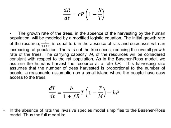
THE BASENER – ROSS MODEL: • Let P be a population and let R be the amount of resources. In this model the carrying capacity is determined by the amount of resources. Those resources are themselves a biological population and are therefore governed by their own standard logistic differential equation. The Basener-Ross model is given by a system of two differential equations. One equation governs the growth rate of the population with the carrying capacity set as R and the second equation governs the growth rate of the resource, R (Basener & Ross, 2004). • To derive the Basener-Ross equations, assume that the resources would equilibrate at their natural carrying capacity in the absence of people. So when the population is zero the equation for the resources should be the standard logistic equation with. As in the standard logistic model above we call c the growth rate and K the carrying capacity of the resources. The constant c has units of inverse time; it is the fraction by which the resource supply would increase per unit time were the resource supply far from the island's carrying capacity. The carrying capacity K has the same units as R, it is the maximum amount of resources that the island can support. • The term -h. P accounts for the harvesting of the resources. The constant h, the person harvesting constant, has units of reciprocal time; it is on the order of the reciprocal of the average lifetime of members of the population. The population P has units of persons, as does R; one unit of the resources is the amount of resources required to support a member of the population through their lifetime. We assume that the resources are accessible so that the amount of harvesting is proportional only to the population. This is a reasonable assumption for people on a small island.

THE INVASIVE SPECIES MODEL: •

THE PARAMETER ESTIMATION: • We will provide estimations of the six parameter values a, b, c, f, h and M. It is impossible to determine the values with precision for an ancient civilization in an ecosystem that no longer exists. Consequently, for each parameter we determine a range of reasonable values using established biological research on similar ecosystems. • The growth rate of the population of people a could reasonably range from 0. 005 to 0. 05 per year. The growth rate for a pre-industrialized civilization tends to be around 0. 0045. (Cohen, 1995) However, in the presence of abundant food this rate can be significantly higher. For example, historically documented cases (Birdsell, 1957) place the growth rate of a human population on Pitcairn Island at 0. 034. • The growth rate of the Polynesian rats c could reasonably range from 5 to 25 per year. A litter size ranges from 1 to 10, with an average of 3. 8. A female rat can have up to 13 litters in a year, with an average of 5. 2. The time to maturity for a female rat is less than one year. (Williams 1973) The sex ratio is usually close to 1: 1, but this changes to a male bias, it seems, in more dense, stable populations. Yearly production rate for females in similar islands are 17. 2 (Hawaii); 9. 8 (Ponape); 4. 8 (Kure), 25. 7 (Malaya) (Tamarin & Malecha, 1972). • It is also worthwhile considering the maximum number of rats that could have been supported on the island. For comparison, the density of rats on Kure Atol, a North Western Hawaiian Island is 45 rats per acre, fluctuating from 30 per acre to 75 per acre. The area of Easter Island is 171 sq-km. , or 42255 acres. Thus, it would be reasonable to observe 2, 000 or more rats on the Easter Island. • We assume that the growth rate of the Rapa Nui Jubaea palm trees could range between 0. 01 per year to 1 per year or more, since each tree produces about 100 kg of nuts per year.

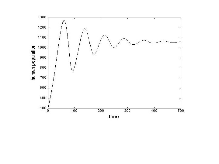
• The Carrying Capacity; It has been estimated that the amount of fertile land needed to supply food for one person is approximately 350 square meters (Cohen, 1995), varying to a great degree on the type of land climate. The area of Easter Island is approximately 166, 000 square meters. If all of it were fertile and if it were farmed efficiently there would be enough food for 475, 000 people. Since only some of the land is farmable and optimal agricultural methods were not being implemented our approximation of a maximum sustainable population of 12, 000 reasonable. We estimate that the carrying capacity of the Rapa Nui Jubaea palm trees in units of people is M = 12, 000. We take this as the carrying capacity for the trees in the absence of people and rats. • Person Harvesting Rate h; It is difficult, perhaps impossible, to get an accurate value for the rate at which the population used the trees. We take h = 0. 25, meaning roughly that every 4 islanders cut down one tree each year. • The Parameter f; The growth rate of the trees is a function of the rat population. The growth rate approaches zero as the rat population approaches infinity. The parameter f is a measure of the decrease in the growth rate of the trees as the number of rat units increases. The growth rate of the trees will be halved when Rf = 1. We estimate that this occurs when R = 1, 000. Thus we estimate f to be approximately 10 -3. • Numerical Simulations; Numerical solutions to the invasive species model with the parameter values taken from the ranges derived above are shown in Figure 1. The parameters used were a = 0. 03, b = 1, c = 10, M = 12, 000, h = 0. 25 and f ranges from 0. 0004 to 0. 001. Observe that, if we assume all parameters other than f are held constant then the rate at which the rats eat nuts determines the long term success or collapse of the human population. The top three traces imply the plausibility of Hunt's hypothesis .

Figure 1: The human population is graphed for f ranging from 0. 0004 to 0. 001. It can be seen that for small values of f the population oscillates around the coexistence equilibrium and for larger values of the f parameter the human population is unstable and crashes. This illustrates that the stability of the coexistence equilibrium in the Invasive Species Model is sensitive to the parameter modeling the effect of the rats.

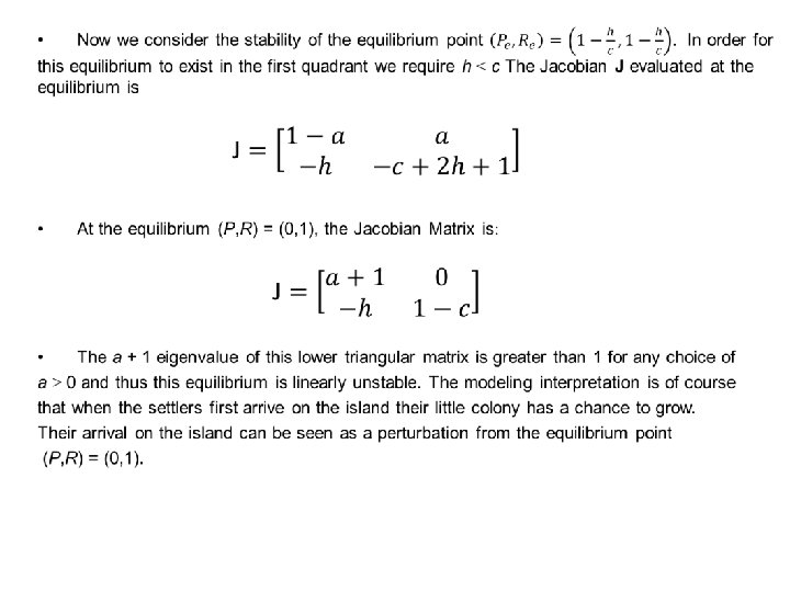
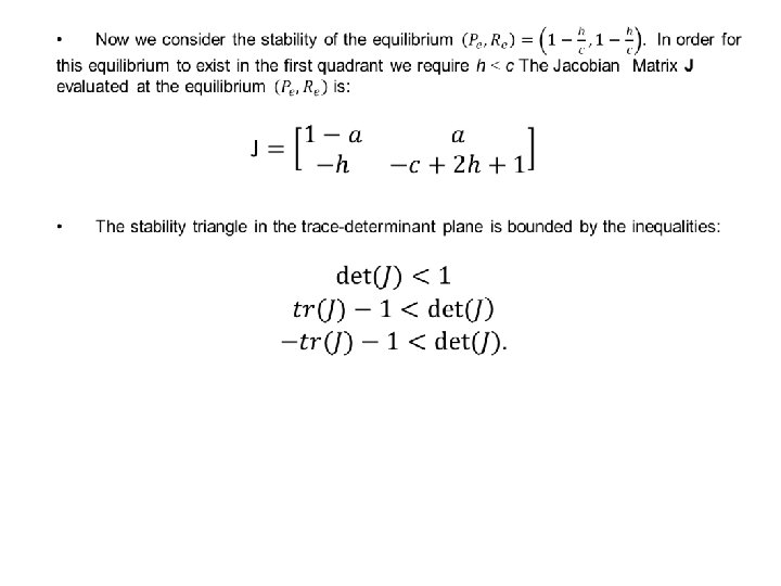
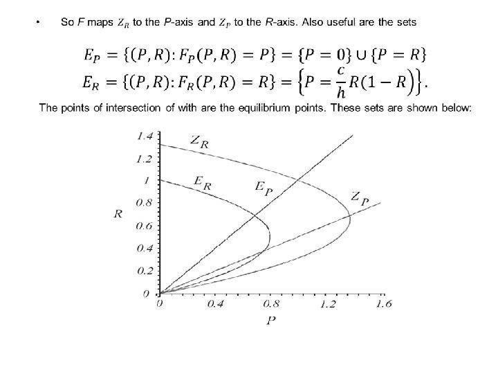
THE EQUILIBRIA OF THE MODEL: •

THE HOPF BIFURCATION AT THE COEXISTENCE EQUILIBRIUM: •

Figure 2: The equation AB = C is implicitly plotted in the parameters h and f. Below the curve the coexistence equilibrium is linearly stable. A Hopf Bifurcation occurs on the curve and above the curve the coexistence equilibrium is linearly unstable. Thus for any level of harvesting by the human population there exists a level of damage that the rats could cause that would crash the human population.

THE DISCRETE MODEL: •

Fig. 3. The graph of population verses time using the discrete model applied to Easter Island. Each 'x' is a data point or data range approximated through archeological evidence. It is important to observe that not only does our model match the archeological data and qualitative description; it does so with realistic parameter values. For example, the 1 -dimensional logistic model can experience a growth and collapse, but not with parameter values close to human growth rates. Moreover, the one dimensional logistic equation could not experience a growth on collapse matching the qualitative timescale provided by archeology for any parameter values.

THE EQUILIBRIA OF THE MODEL: •

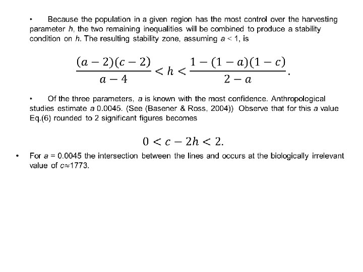
Fig. 4. The stability region for a = 0. 0045, a = 0. 3, and a = 1.

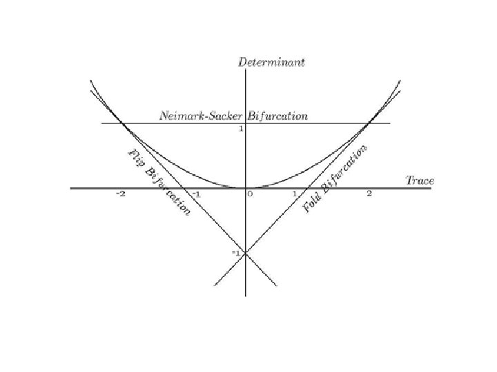
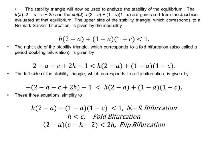
The Neimark-Sacker Bifurcation: •

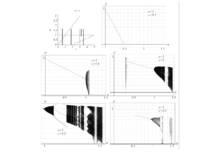
Fig. 5. Three phase planes are shown with a = 0. 0045, c = 3 and h-values near the Neimark-Sacker bifurcation.

Numerical Bifurcation Analysis: Fig. 6. The first plot is the stability region in the c, h-parameter plane for a = 0. 0045 with lines indicating the parameter values for the bifurcation diagrams. Bifurcation diagrams are shown for a = 0. 0045 with c = 0. 5, c = 1. 8, and c = 3.

Fig. 5. The first 1000 iterates of 5000 initial conditions for a = 0. 0045, c = 3 and h = 0. 15 and h = 1. These parameter values are indicated by the arrows in the bifurcation diagram in Fig. 6. In the case with h = 0. 15 the attractor is a chaotic region indicated by the arrow. In the case with h = 1 the attractor is an equilibrium point, also indicated by an arrow. In each case, the set resembling a bifurcation diagram for the logistic equation forms a ``stable set'' for the attractor.

Fig. 6. The first plot is the stability region in the c, h-parameter plane for a = 0. 3 with lines indicating the parameter values for the bifurcation diagrams. Bifurcation diagrams are shown for a = 0. 3 with c = 0. 5, c = 1. 8, and c = 3. Observe the nontrivial attractors that occur just outside the stability region.

Fig. 7. The attractor for the system with a = 1, c = 3. 5, and h = 1. 5.

Global Analysis and Basins of Attraction: •

The Julia Set: •

Fig. 8. The Julia set for a = 1, c = 3. 2, and h = 0. 9.

Fig. 9. The Julia set for a = 1, c = 3. 2, and h = 0. 9 showing the escape sets.

THE DIFFUSION: •

THE DECOUPLED FORM OF THE EQUATIONS: •

Fig. 10: The left plot illustrates the stability of the interior coexistence equilibrium when DR = 0. 15 and the right plot illustrates the Turing instability that occurs using the same initial conditions but with DR = 0. 17. The dashed line is the human population and the solid line is the rat population.

Fig. 11: The plot on the previous page shows the total Island population reaching a stable interior coexistence equilibrium of people whereas the plot on this page shows the crash of the total Island population caused by increased rat mobility.