Dynamics 101 Jim Van Verth Red Storm Entertainment

Dynamics 101 Jim Van Verth > Red Storm Entertainment > jimvv@redstorm. com >

What is Dynamics? Want to move objects through the game world in the most realistic manner possible > Applying velocity not enough – need ramp up, ramp down – acceleration > Same with orientation >

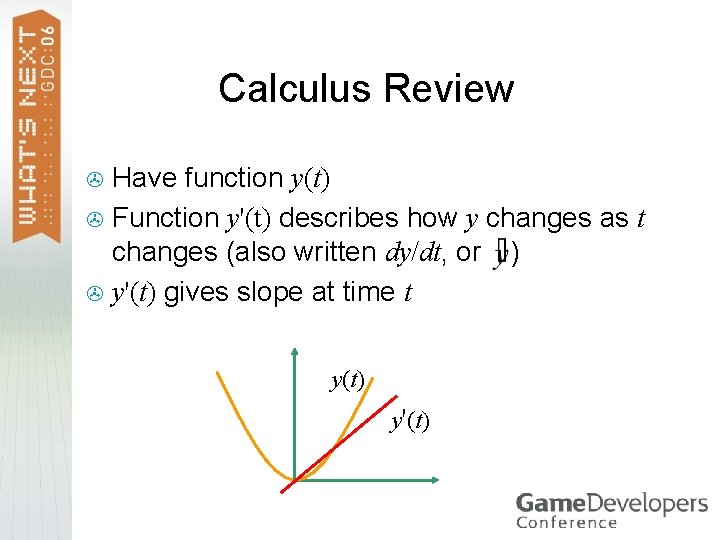
Calculus Review Have function y(t) > Function y'(t) describes how y changes as t changes (also written dy/dt, or ) > y'(t) gives slope at time t > y y(t) y'(t) t

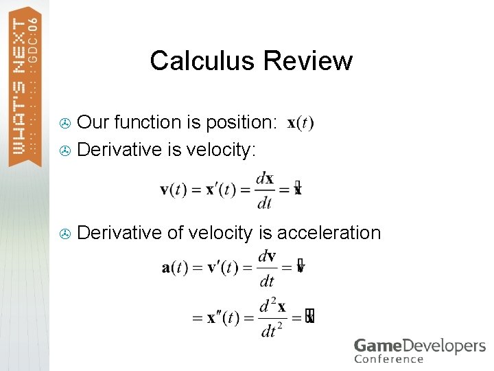
Calculus Review Our function is position: > Derivative is velocity: > > Derivative of velocity is acceleration

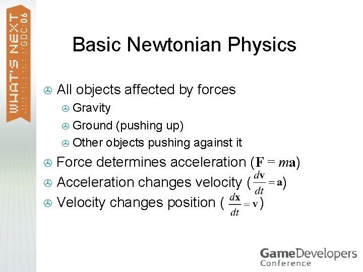
Basic Newtonian Physics > All objects affected by forces Gravity > Ground (pushing up) > Other objects pushing against it > Force determines acceleration (F = ma) > Acceleration changes velocity ( ) > Velocity changes position ( ) >

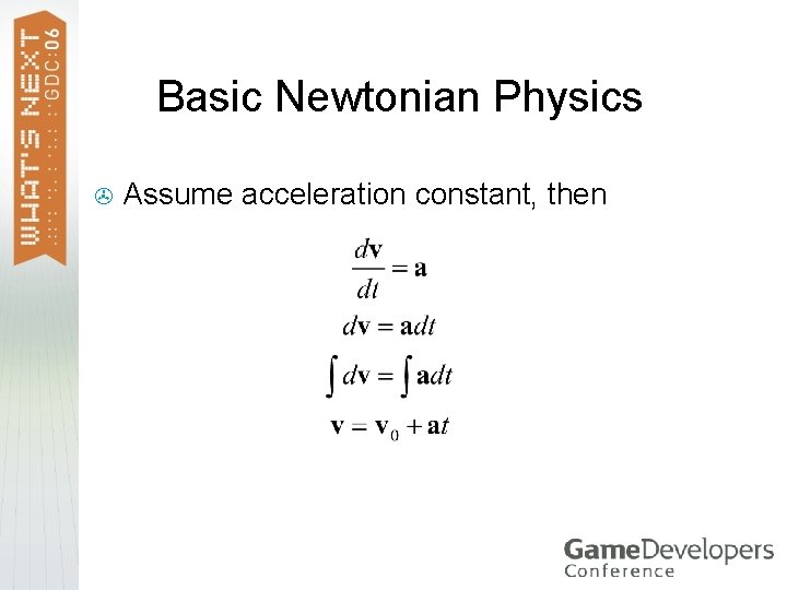
Basic Newtonian Physics > Assume acceleration constant, then

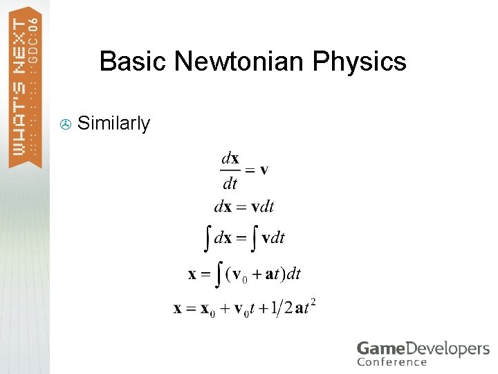
Basic Newtonian Physics > Similarly

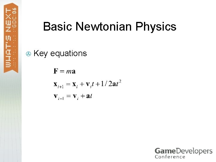
Basic Newtonian Physics > Key equations

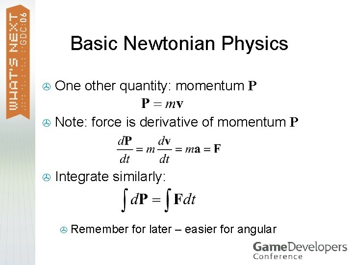
Basic Newtonian Physics > One other quantity: momentum P > Note: force is derivative of momentum P > Integrate similarly: > Remember for later – easier for angular

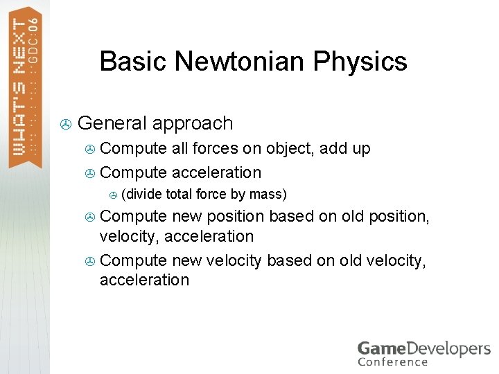
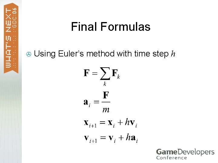
Basic Newtonian Physics > General approach Compute all forces on object, add up > Compute acceleration > > (divide total force by mass) Compute new position based on old position, velocity, acceleration > Compute new velocity based on old velocity, acceleration >

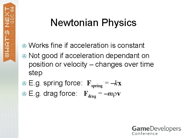
Newtonian Physics Works fine if acceleration is constant > Not good if acceleration dependant on position or velocity – changes over time step > E. g. spring force: Fspring = –kx > E. g. drag force: Fdrag = –m v >

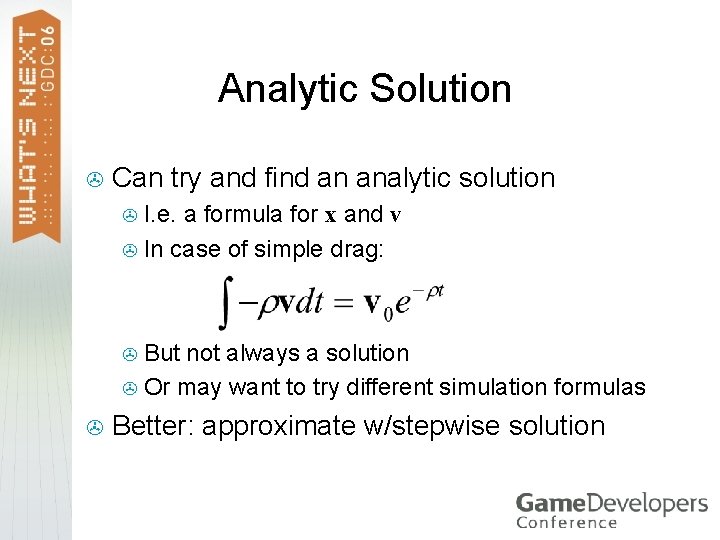
Analytic Solution > Can try and find an analytic solution I. e. a formula for x and v > In case of simple drag: > But not always a solution > Or may want to try different simulation formulas > > Better: approximate w/stepwise solution

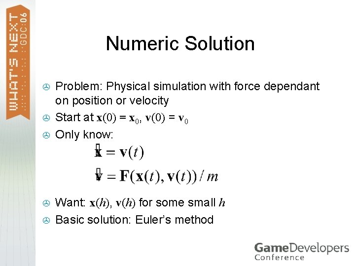
Numeric Solution > > > Problem: Physical simulation with force dependant on position or velocity Start at x(0) = x 0, v(0) = v 0 Only know: Want: x(h), v(h) for some small h Basic solution: Euler’s method

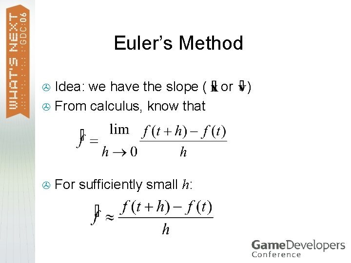
Euler’s Method Idea: we have the slope ( > From calculus, know that > > For sufficiently small h: or )

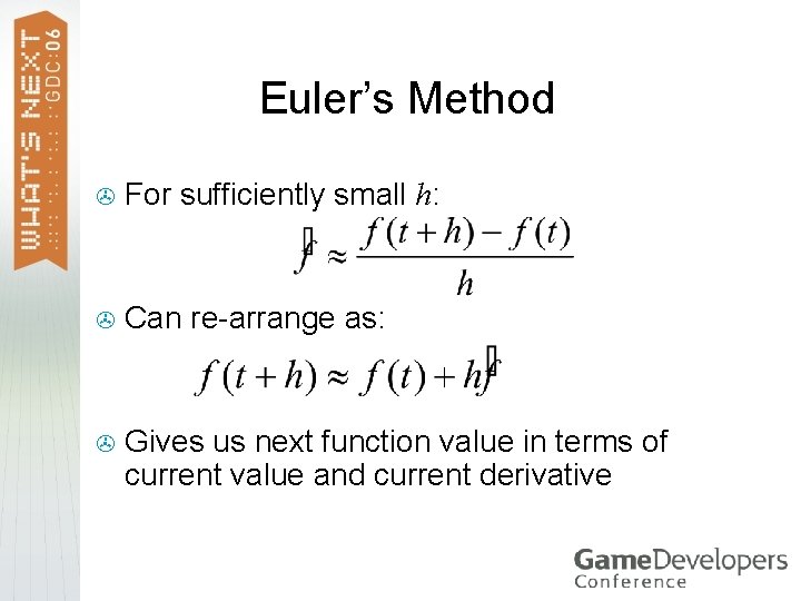
Euler’s Method > For sufficiently small h: > Can re-arrange as: > Gives us next function value in terms of current value and current derivative

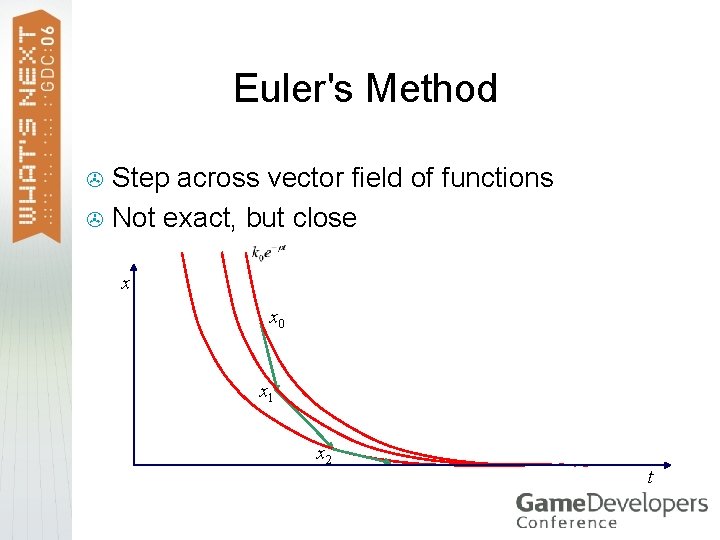
Euler's Method Step across vector field of functions > Not exact, but close > x x 0 x 1 x 2 t

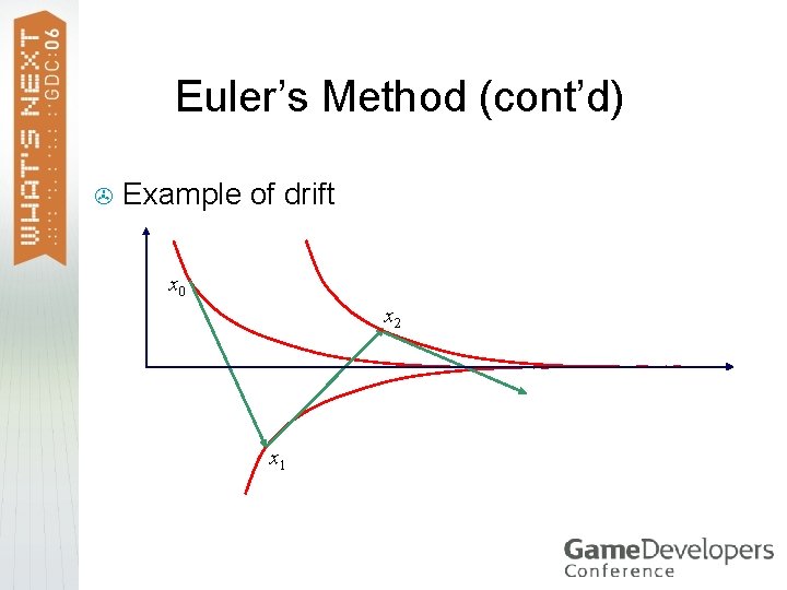
Euler’s Method > Has problems Expects the slope at the current point is a good estimate of the slope on the interval > Approximation can drift off the actual function – adds energy to system! > Gets worse the farther we get from known initial value > Especially bad when time step gets larger >

Euler’s Method (cont’d) > Example of drift x x 0 x 2 t x 1

Stiffness Running into classic problem of stiff equations > Have terms with rapidly decaying values > Faster decay = stiffer equation = need smaller h > Often seen in equations with stiff springs (hence the name) >

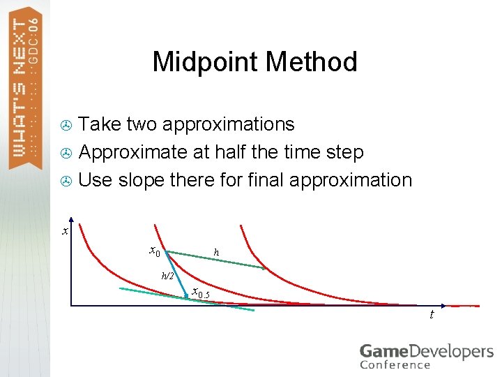
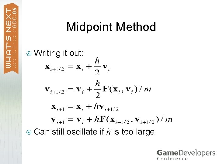
Midpoint Method Take two approximations > Approximate at half the time step > Use slope there for final approximation > x x 0 h h/2 x 1 x 0. 5 t

Midpoint Method > Writing it out: > Can still oscillate if h is too large

Runge-Kutta Use weighted average of slopes across interval > How error-resistant indicates order > Midpoint method is order two > Usually use Runge-Kutta Order Four, or RK 4 >

Runge-Kutta (cont’d) Better fit, good for larger time steps > Expensive – requires many evaluations > If function is known and fixed (like in physical simulation) can reduce it to one big formula > But for large timesteps, still have trouble with stiff equations >

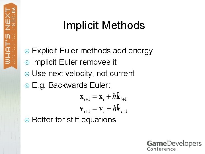
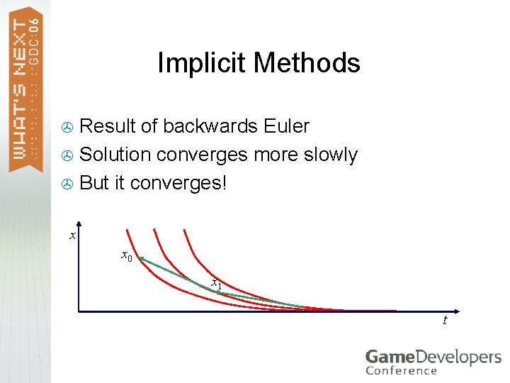
Implicit Methods Explicit Euler methods add energy > Implicit Euler removes it > Use next velocity, not current > E. g. Backwards Euler: > > Better for stiff equations

Implicit Methods Result of backwards Euler > Solution converges more slowly > But it converges! > x x 0 x 1 x 2 t

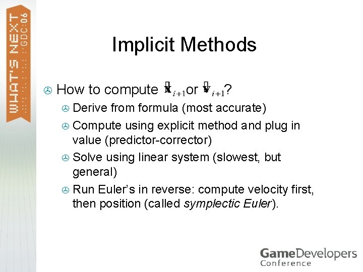
Implicit Methods > How to compute or ? Derive from formula (most accurate) > Compute using explicit method and plug in value (predictor-corrector) > Solve using linear system (slowest, but general) > Run Euler’s in reverse: compute velocity first, then position (called symplectic Euler). >

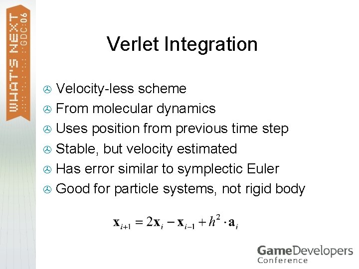
Verlet Integration Velocity-less scheme > From molecular dynamics > Uses position from previous time step > Stable, but velocity estimated > Has error similar to symplectic Euler > Good for particle systems, not rigid body >

Which To Use? In practice, Midpoint or Euler’s method may be enough if time step is small > At 60 fps, that’s probably the case > In case of long frame times, can clamp simulation time step to 1/10 sec > Having trouble w/sim exploding? Try symplectic Euler or Verlet >

Final Formulas > Using Euler’s method with time step h

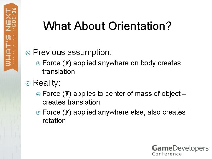
What About Orientation? > Previous assumption: > > Force (F) applied anywhere on body creates translation Reality: Force (F) applies to center of mass of object – creates translation > Force (F) applied anywhere else, also creates rotation >

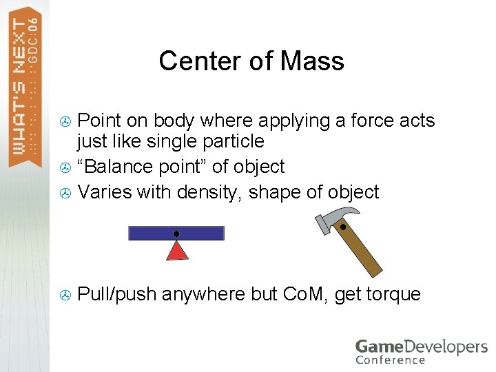
Center of Mass Point on body where applying a force acts just like single particle > “Balance point” of object > Varies with density, shape of object > > Pull/push anywhere but Co. M, get torque

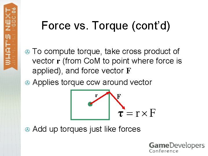
Force vs. Torque (cont’d) To compute torque, take cross product of vector r (from Co. M to point where force is applied), and force vector F > Applies torque ccw around vector > F Add up torques just like forces

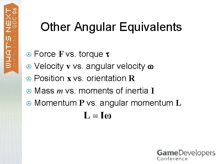
Other Angular Equivalents Force F vs. torque > Velocity v vs. angular velocity > Position x vs. orientation R > Mass m vs. moments of inertia I > Momentum P vs. angular momentum L >

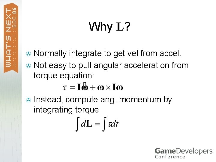
Why L? Normally integrate to get vel from accel. > Not easy to pull angular acceleration from torque equation: > > Instead, compute ang. momentum by integrating torque

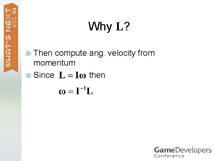
Why L? Then compute ang. velocity from momentum > Since then >

Moments of Inertia Moments of inertia are 3 x 3 matrix, not single scalar factor (unlike m) > Many factors because rotation depends on shape > Describe how object rotates around various axes > Not always easy to compute > Change as object changes orientation >

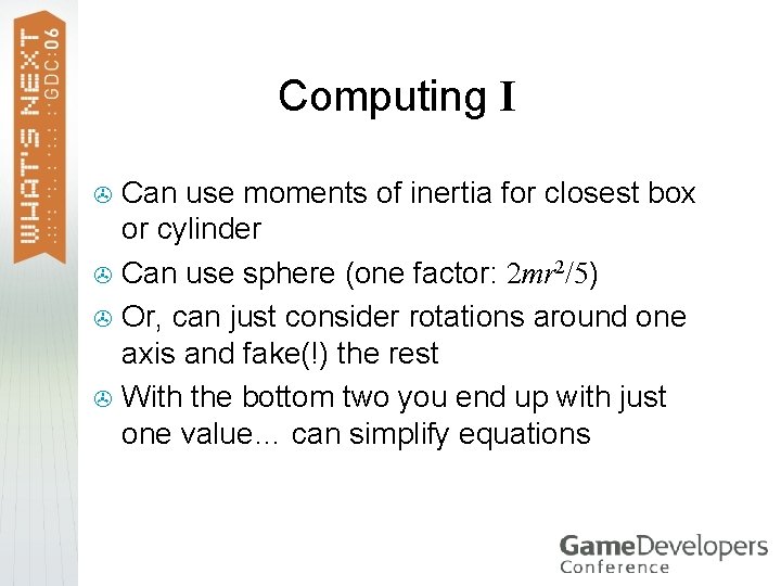
Computing I Can use moments of inertia for closest box or cylinder > Can use sphere (one factor: 2 mr 2/5) > Or, can just consider rotations around one axis and fake(!) the rest > With the bottom two you end up with just one value… can simplify equations >

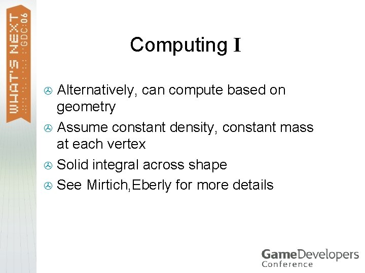
Computing I Alternatively, can compute based on geometry > Assume constant density, constant mass at each vertex > Solid integral across shape > See Mirtich, Eberly for more details >

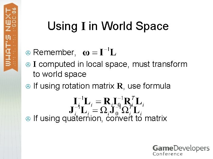
Using I in World Space Remember, > I computed in local space, must transform to world space > If using rotation matrix R, use formula > > If using quaternion, convert to matrix

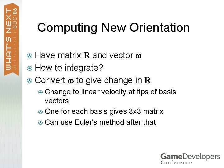
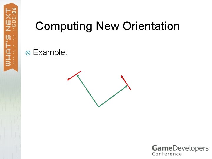
Computing New Orientation Have matrix R and vector > How to integrate? > Convert to give change in R > Change to linear velocity at tips of basis vectors > One for each basis gives 3 x 3 matrix > Can use Euler's method after that >

Computing New Orientation > Example:

Computing New Orientation r gives linear velocity at r > Could do this for each basis vector > Better way: > Use symmetric skew matrix to compute cross products > Multiply by orientation matrix >

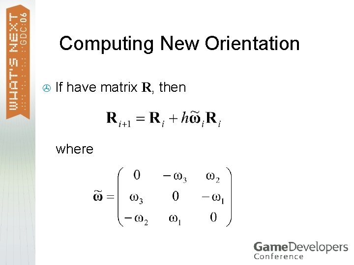
Computing New Orientation > If have matrix R, then where

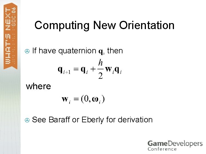
Computing New Orientation > If have quaternion q, then where > See Baraff or Eberly for derivation

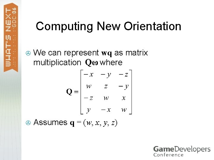
Computing New Orientation > We can represent wq as matrix multiplication where > Assumes q = (w, x, y, z)

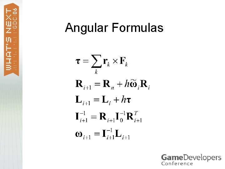
Angular Formulas

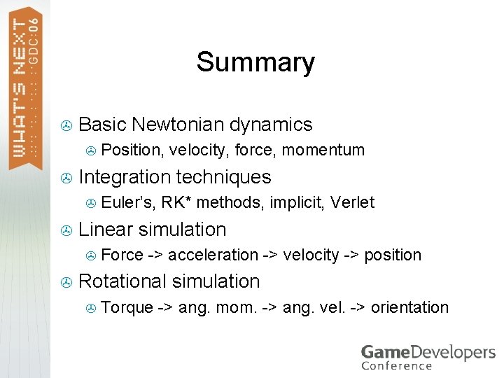
Summary > Basic Newtonian dynamics > > Integration techniques > > Euler’s, RK* methods, implicit, Verlet Linear simulation > > Position, velocity, force, momentum Force -> acceleration -> velocity -> position Rotational simulation > Torque -> ang. mom. -> ang. vel. -> orientation

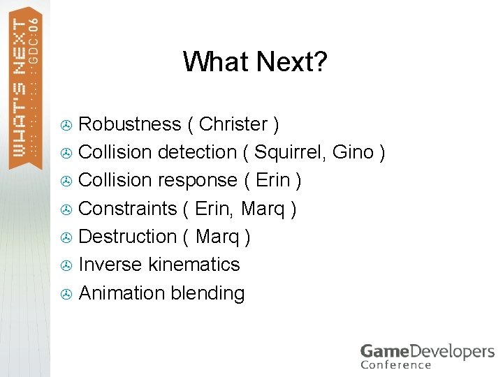
What Next? Robustness ( Christer ) > Collision detection ( Squirrel, Gino ) > Collision response ( Erin ) > Constraints ( Erin, Marq ) > Destruction ( Marq ) > Inverse kinematics > Animation blending >

References > > Burden, Richard L. and J. Douglas Faires, Numerical Analysis, PWS Publishing Company, Boston, MA, 1993. Hecker, Chris, “Behind the Screen, ” Game Developer, Miller Freeman, San Francisco, Dec. 1996 -Jun. 1997. Witken, Andrew, David Baraff, Michael Kass, SIGGRAPH Course Notes, Physically Based Modelling, SIGGRAPH 2002. Eberly, David, Game Physics, Morgan Kaufmann, 2003.