Dynamical Systems 1 Introduction Ing Jaroslav Jra CSc

Dynamical Systems 1 Introduction Ing. Jaroslav Jíra, CSc.

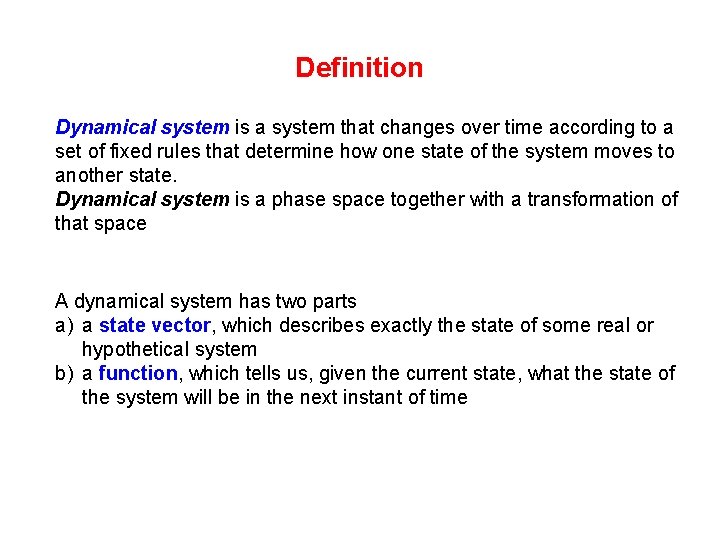
Definition Dynamical system is a system that changes over time according to a set of fixed rules that determine how one state of the system moves to another state. Dynamical system is a phase space together with a transformation of that space A dynamical system has two parts a) a state vector, which describes exactly the state of some real or hypothetical system b) a function, which tells us, given the current state, what the state of the system will be in the next instant of time

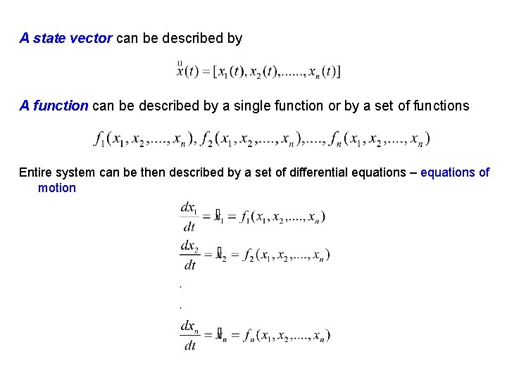
A state vector can be described by A function can be described by a single function or by a set of functions Entire system can be then described by a set of differential equations – equations of motion

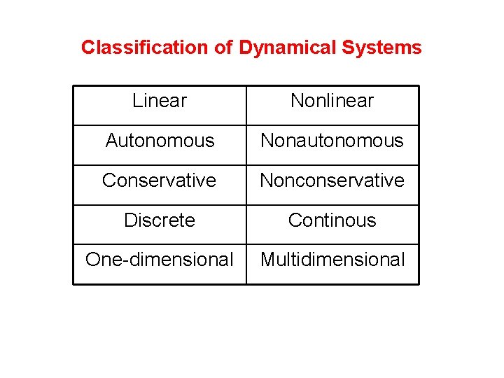
Classification of Dynamical Systems Linear Nonlinear Autonomous Nonautonomous Conservative Nonconservative Discrete Continous One-dimensional Multidimensional

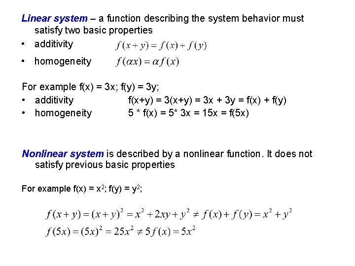
Linear system – a function describing the system behavior must satisfy two basic properties • additivity • homogeneity For example f(x) = 3 x; f(y) = 3 y; • additivity f(x+y) = 3 x + 3 y = f(x) + f(y) • homogeneity 5 * f(x) = 5* 3 x = 15 x = f(5 x) Nonlinear system is described by a nonlinear function. It does not satisfy previous basic properties For example f(x) = x 2; f(y) = y 2;

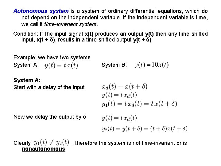
Autonomous system is a system of ordinary differential equations, which do not depend on the independent variable. If the independent variable is time, we call it time-invariant system. Condition: If the input signal x(t) produces an output y(t) then any time shifted input, x(t + δ), results in a time-shifted output y(t + δ) Example: we have two systems System A: System B: System A: Start with a delay of the input Now we delay the output by δ Clearly nonautonomous. , therefore the system is not time-invariant or is

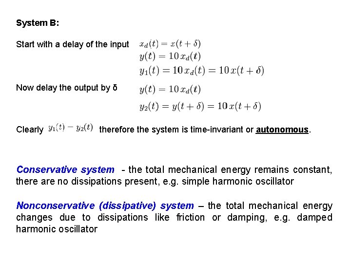
System B: Start with a delay of the input Now delay the output by δ Clearly therefore the system is time-invariant or autonomous. Conservative system - the total mechanical energy remains constant, there are no dissipations present, e. g. simple harmonic oscillator Nonconservative (dissipative) system – the total mechanical energy changes due to dissipations like friction or damping, e. g. damped harmonic oscillator

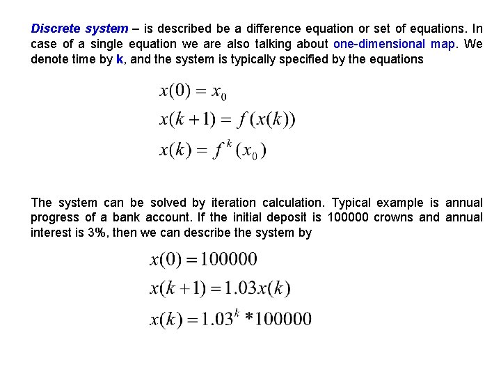
Discrete system – is described be a difference equation or set of equations. In case of a single equation we are also talking about one-dimensional map. We denote time by k, and the system is typically specified by the equations The system can be solved by iteration calculation. Typical example is annual progress of a bank account. If the initial deposit is 100000 crowns and annual interest is 3%, then we can describe the system by

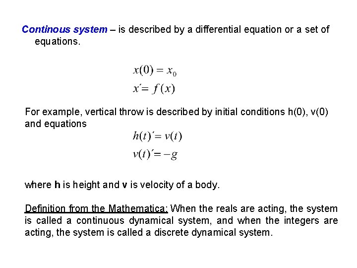
Continous system – is described by a differential equation or a set of equations. For example, vertical throw is described by initial conditions h(0), v(0) and equations where h is height and v is velocity of a body. Definition from the Mathematica: When the reals are acting, the system is called a continuous dynamical system, and when the integers are acting, the system is called a discrete dynamical system.

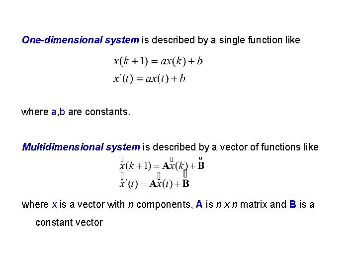
One-dimensional system is described by a single function like where a, b are constants. Multidimensional system is described by a vector of functions like where x is a vector with n components, A is n x n matrix and B is a constant vector

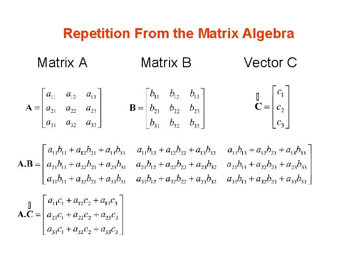
Repetition From the Matrix Algebra Matrix A Matrix B Vector C

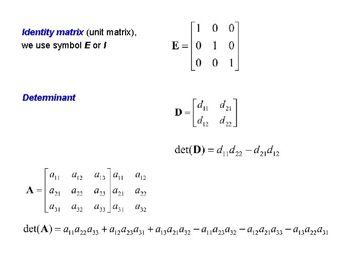
Identity matrix (unit matrix), we use symbol E or I Determinant

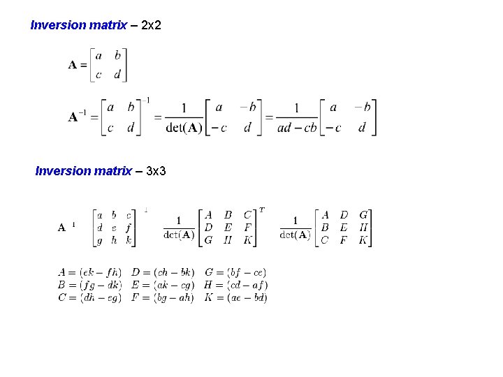
Inversion matrix – 2 x 2 Inversion matrix – 3 x 3

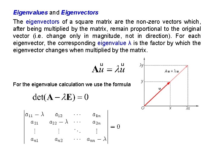
Eigenvalues and Eigenvectors The eigenvectors of a square matrix are the non-zero vectors which, after being multiplied by the matrix, remain proportional to the original vector (i. e. change only in magnitude, not in direction). For each eigenvector, the corresponding eigenvalue λ is the factor by which the eigenvector changes when multiplied by the matrix. For the eigenvalue calculation we use the formula

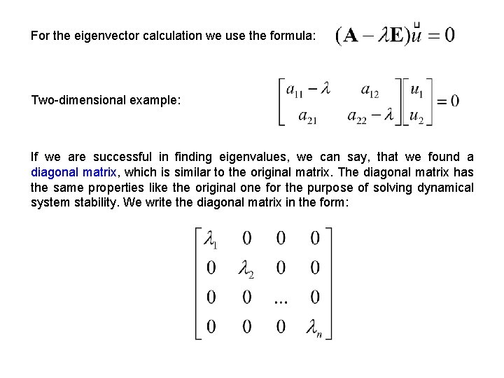
For the eigenvector calculation we use the formula: Two-dimensional example: If we are successful in finding eigenvalues, we can say, that we found a diagonal matrix, which is similar to the original matrix. The diagonal matrix has the same properties like the original one for the purpose of solving dynamical system stability. We write the diagonal matrix in the form:

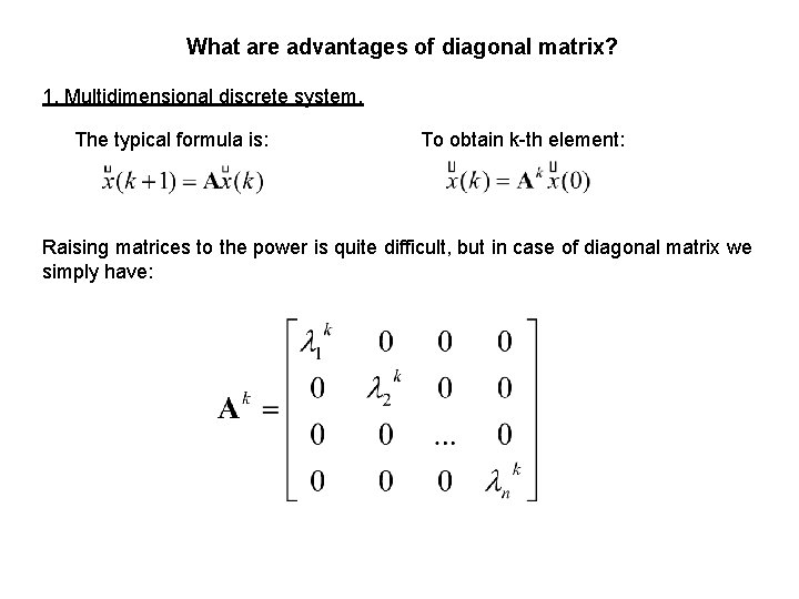
What are advantages of diagonal matrix? 1. Multidimensional discrete system. The typical formula is: To obtain k-th element: Raising matrices to the power is quite difficult, but in case of diagonal matrix we simply have:

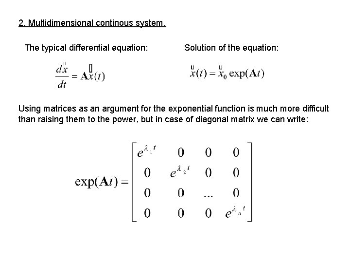
2. Multidimensional continous system. The typical differential equation: Solution of the equation: Using matrices as an argument for the exponential function is much more difficult than raising them to the power, but in case of diagonal matrix we can write:

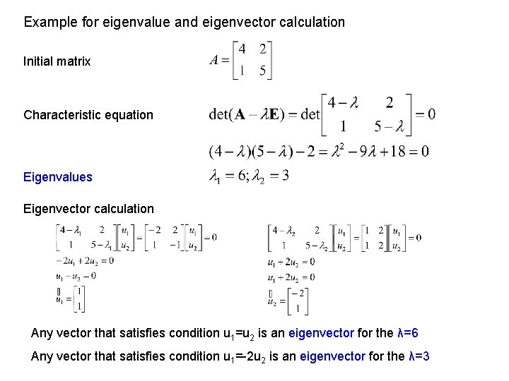
Example for eigenvalue and eigenvector calculation Initial matrix Characteristic equation Eigenvalues Eigenvector calculation Any vector that satisfies condition u 1=u 2 is an eigenvector for the λ=6 Any vector that satisfies condition u 1=-2 u 2 is an eigenvector for the λ=3

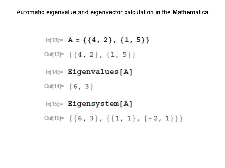
Automatic eigenvalue and eigenvector calculation in the Mathematica

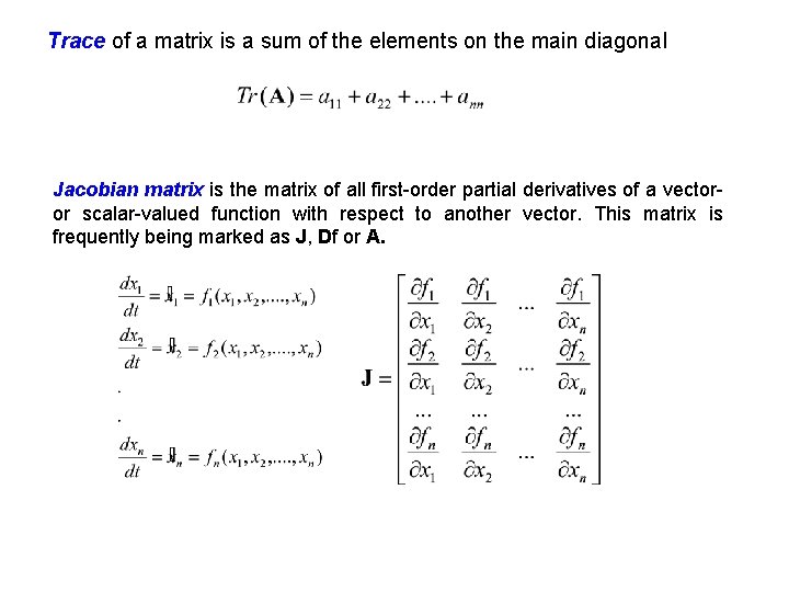
Trace of a matrix is a sum of the elements on the main diagonal Jacobian matrix is the matrix of all first-order partial derivatives of a vectoror scalar-valued function with respect to another vector. This matrix is frequently being marked as J, Df or A.

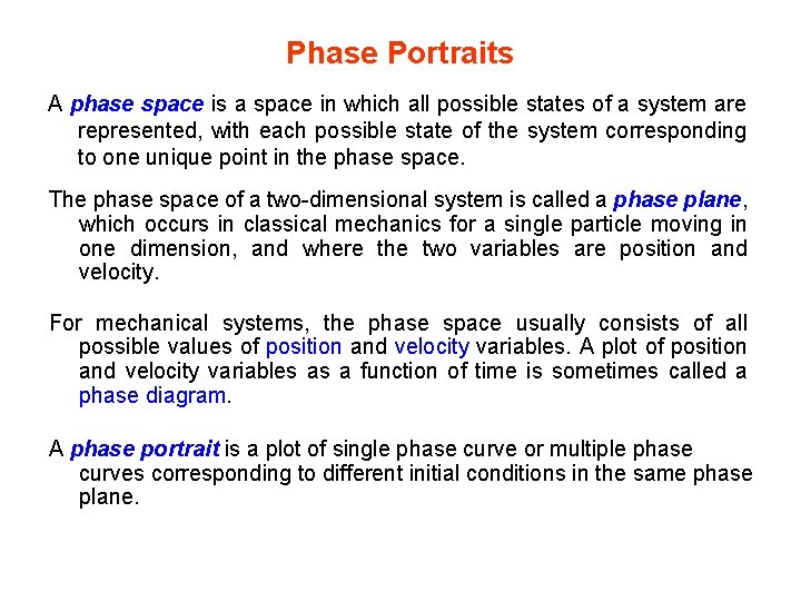
Phase Portraits A phase space is a space in which all possible states of a system are represented, with each possible state of the system corresponding to one unique point in the phase space. The phase space of a two-dimensional system is called a phase plane, which occurs in classical mechanics for a single particle moving in one dimension, and where the two variables are position and velocity. For mechanical systems, the phase space usually consists of all possible values of position and velocity variables. A plot of position and velocity variables as a function of time is sometimes called a phase diagram. A phase portrait is a plot of single phase curve or multiple phase curves corresponding to different initial conditions in the same phase plane.

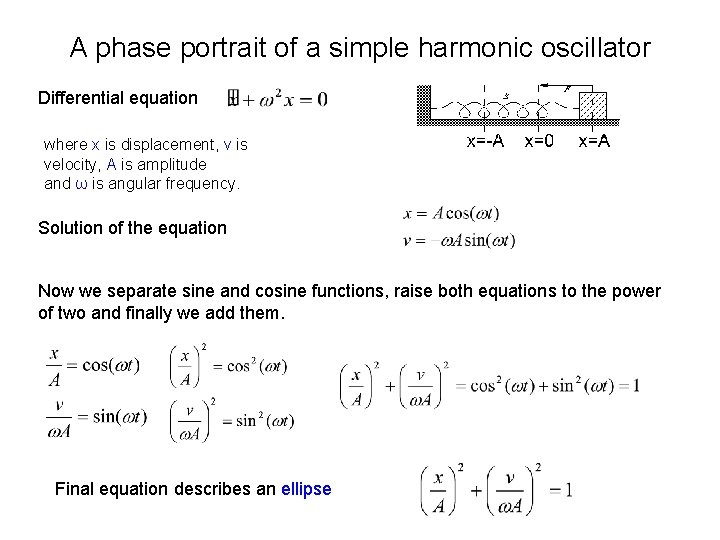
A phase portrait of a simple harmonic oscillator Differential equation where x is displacement, v is velocity, A is amplitude and ω is angular frequency. Solution of the equation Now we separate sine and cosine functions, raise both equations to the power of two and finally we add them. Final equation describes an ellipse

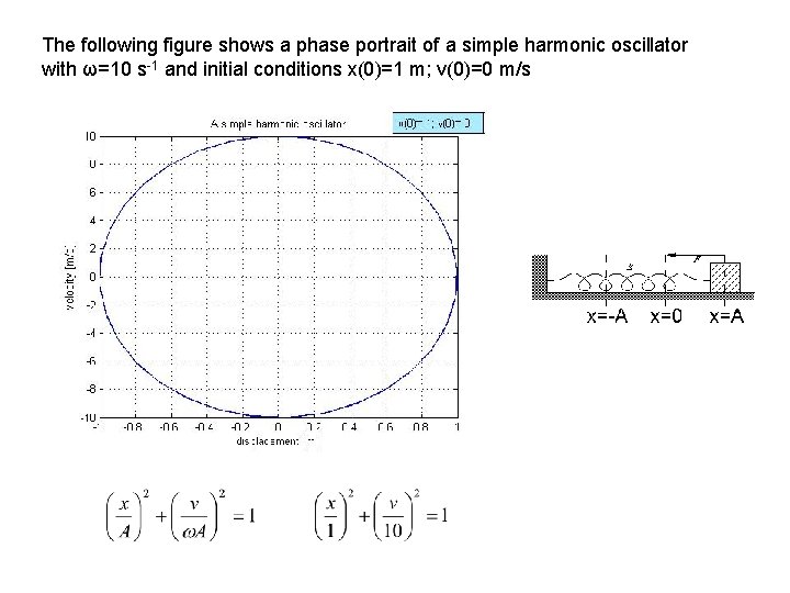
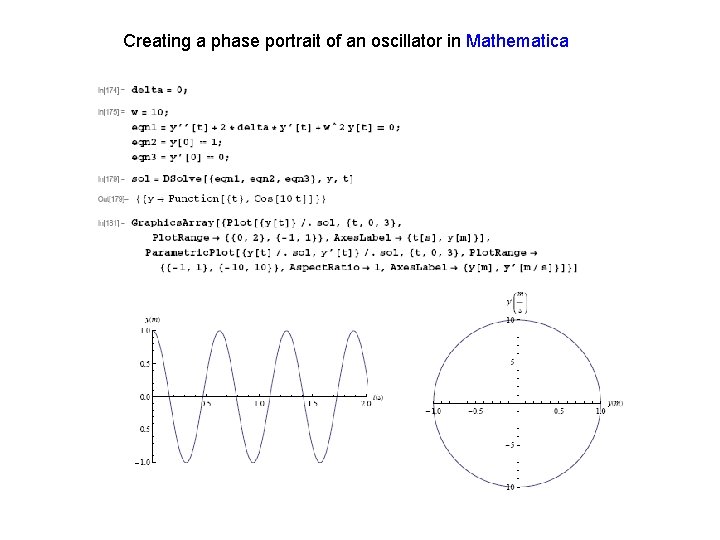
The following figure shows a phase portrait of a simple harmonic oscillator with ω=10 s-1 and initial conditions x(0)=1 m; v(0)=0 m/s

Creating a phase portrait of a damped oscillator in Matlab function [t, y] = oscil(delta) tspan=[0, 7]; init=[1; 0]; omega=10; [t, y]=ode 45(@f, tspan, init); plot(y(: , 1), y(: , 2)); %Creation of graph description. xlabel('displacement [m]') ylabel('velocity [m/s]') title('A damped harmonic oscillator'); axis([-1 1 -10 10]); function yprime=f(t, y) yprime=zeros(2, 1); yprime(1)=y(2); yprime(2)=-2*delta*y(2)-omega^2*y(1); end clc end

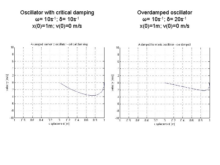
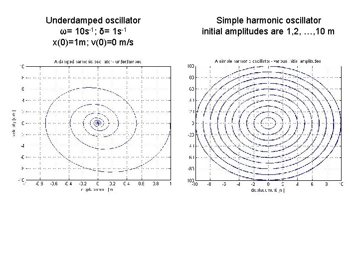
Oscillator with critical damping ω= 10 s-1; δ= 10 s-1 x(0)=1 m; v(0)=0 m/s Overdamped oscillator ω= 10 s-1; δ= 20 s-1 x(0)=1 m; v(0)=0 m/s

Underdamped oscillator ω= 10 s-1; δ= 1 s-1 x(0)=1 m; v(0)=0 m/s Simple harmonic oscillator initial amplitudes are 1, 2, …, 10 m

Creating a phase portrait of an oscillator in Mathematica

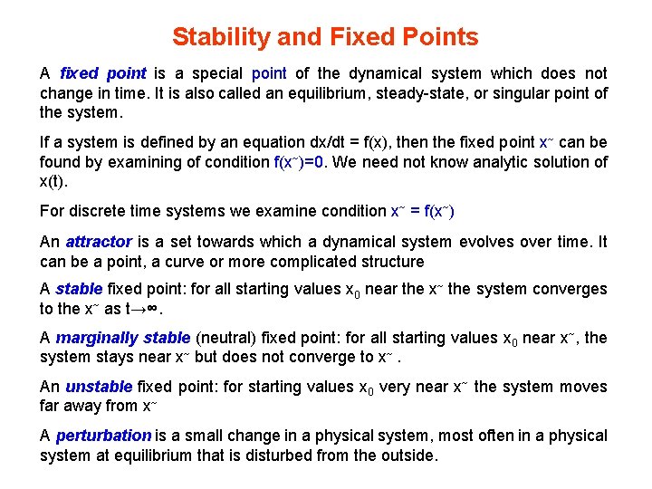
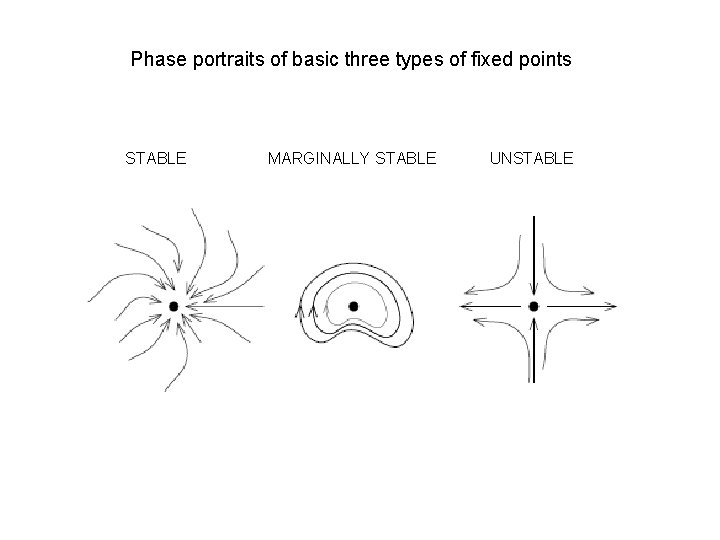
Stability and Fixed Points A fixed point is a special point of the dynamical system which does not change in time. It is also called an equilibrium, steady-state, or singular point of the system. If a system is defined by an equation dx/dt = f(x), then the fixed point x~ can be found by examining of condition f(x~)=0. We need not know analytic solution of x(t). For discrete time systems we examine condition x~ = f(x~) An attractor is a set towards which a dynamical system evolves over time. It can be a point, a curve or more complicated structure A stable fixed point: for all starting values x 0 near the x~ the system converges to the x~ as t→∞. A marginally stable (neutral) fixed point: for all starting values x 0 near x~, the system stays near x~ but does not converge to x~. An unstable fixed point: for starting values x 0 very near x~ the system moves far away from x~ A perturbation is a small change in a physical system, most often in a physical system at equilibrium that is disturbed from the outside.

Phase portraits of basic three types of fixed points STABLE MARGINALLY STABLE UNSTABLE

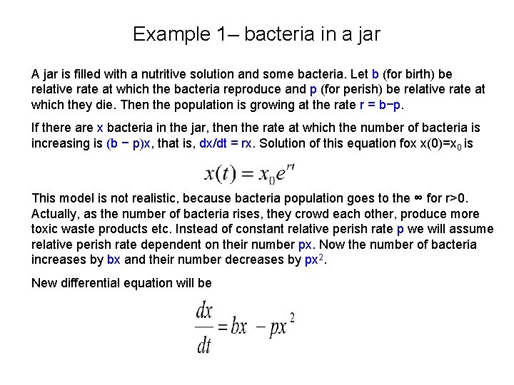
Example 1– bacteria in a jar A jar is filled with a nutritive solution and some bacteria. Let b (for birth) be relative rate at which the bacteria reproduce and p (for perish) be relative rate at which they die. Then the population is growing at the rate r = b−p. If there are x bacteria in the jar, then the rate at which the number of bacteria is increasing is (b − p)x, that is, dx/dt = rx. Solution of this equation fox x(0)=x 0 is This model is not realistic, because bacteria population goes to the ∞ for r>0. Actually, as the number of bacteria rises, they crowd each other, produce more toxic waste products etc. Instead of constant relative perish rate p we will assume relative perish rate dependent on their number px. Now the number of bacteria increases by bx and their number decreases by px 2. New differential equation will be

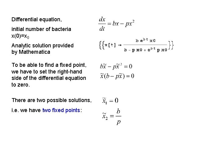
Differential equation, initial number of bacteria x(0)=x 0 Analytic solution provided by Mathematica To be able to find a fixed point, we have to set the right-hand side of the differential equation to zero. There are two possible solutions, i. e. we have two fixed points:

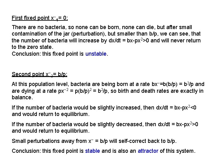
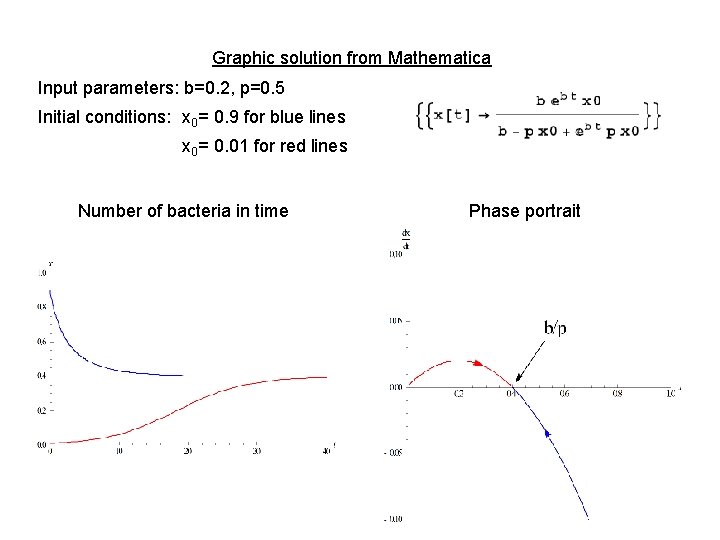
First fixed point x~1= 0; There are no bacteria, so none can be born, none can die, but after small contamination of the jar (perturbation), but smaller than b/p, we can see, that the number of bacteria will increase by dx/dt = bx-px 2>0 and will never return to the zero state. Conclusion: this fixed point is unstable. Second point x~2= b/p; At this population level, bacteria are being born at a rate bx~=b(b/p) = b 2/p and are dying at a rate px~2 = p(b/p)2 = b 2/p, so birth and death rates are exactly in balance. If the number of bacteria would be slightly increased, then dx/dt = bx-px 2<0 and would return to equilibrium. If the number of bacteria would be slightly decreased, then dx/dt = bx-px 2>0 and would return to equilibrium. Small perturbations away from x~ = b/p will self-correct back to b/p. Conclusion: this fixed point is stable and is also an attractor of this system.

Graphic solution from Mathematica Input parameters: b=0. 2, p=0. 5 Initial conditions: x 0= 0. 9 for blue lines x 0= 0. 01 for red lines Number of bacteria in time Phase portrait

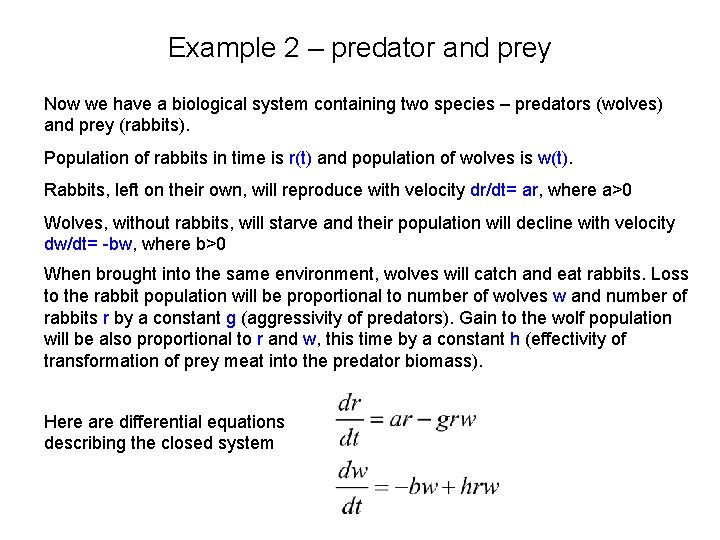
Example 2 – predator and prey Now we have a biological system containing two species – predators (wolves) and prey (rabbits). Population of rabbits in time is r(t) and population of wolves is w(t). Rabbits, left on their own, will reproduce with velocity dr/dt= ar, where a>0 Wolves, without rabbits, will starve and their population will decline with velocity dw/dt= -bw, where b>0 When brought into the same environment, wolves will catch and eat rabbits. Loss to the rabbit population will be proportional to number of wolves w and number of rabbits r by a constant g (aggressivity of predators). Gain to the wolf population will be also proportional to r and w, this time by a constant h (effectivity of transformation of prey meat into the predator biomass). Here are differential equations describing the closed system

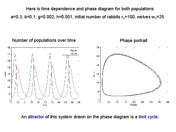
Here is time dependence and phase diagram for both populations a=0. 3; b=0. 1; g=0. 002; h=0. 001, initial number of rabbits r 0=100, wolves w 0=25 Number of populations over time Phase portrait An attractor of this system drawn on the phase diagram is a limit cycle.

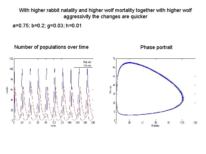
With higher rabbit natality and higher wolf mortality together with higher wolf aggressivity the changes are quicker a=0. 75; b=0. 2; g=0. 03; h=0. 01 Number of populations over time Phase portrait

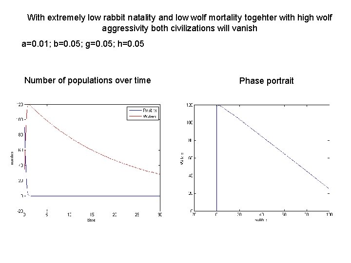
With extremely low rabbit natality and low wolf mortality togehter with high wolf aggressivity both civilizations will vanish a=0. 01; b=0. 05; g=0. 05; h=0. 05 Number of populations over time Phase portrait

Source codes from Matlab for both types of graphs function [t, x, y] = predatorparam a=0. 2; b=0. 1; g=0. 002; h=0. 001; tend=200; x 0 = [100; 25]; [t, xvec] = ode 45(@f, [0, tend], x 0); x = xvec(: , 1); y = xvec(: , 2); % Plot of the solution p=plot(t, x, t, y); xlabel('time'); ylabel('number'); hleg = legend('Rabbits', 'Wolves'); % Plot of the solution p=plot(x, y); xlabel('Rabbits'); ylabel('Wolves'); function xdot = f(t, x) xdot= [ a*x(1) - g*x(1)*x(2); . . . -b*x(2) + h*x(1)*x(2)]; end end