Dynamical Springslider Lattice Models for Earthquake Faults JeenHwa

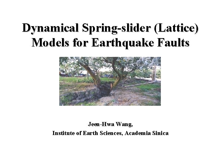
Dynamical Spring-slider (Lattice) Models for Earthquake Faults Jeen-Hwa Wang, Institute of Earth Sciences, Academia Sinica

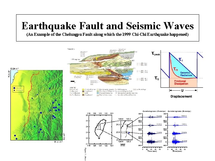
Earthquake Fault and Seismic Waves (An Example of the Chelungpu Fault along which the 1999 Chi-Chi Earthquake happened)

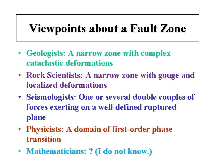
Viewpoints about a Fault Zone • Geologists: A narrow zone with complex cataclastic deformations • Rock Scientists: A narrow zone with gouge and localized deformations • Seismologists: One or several double couples of forces exerting on a well-defined ruptured plane • Physicists: A domain of first-order phase transition • Mathematicians: ? (I do not know. )

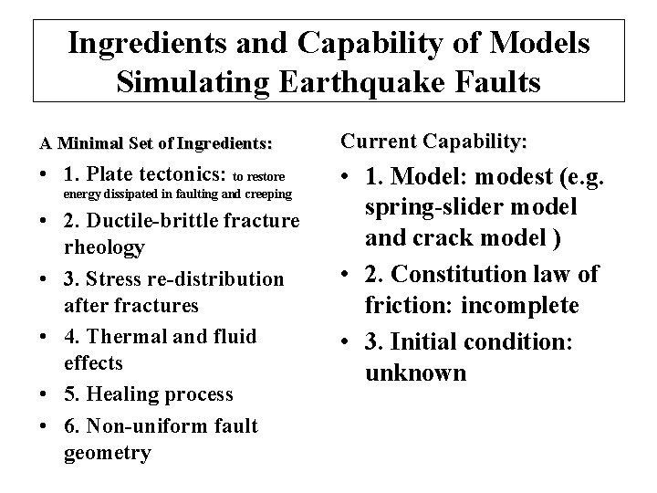
Ingredients and Capability of Models Simulating Earthquake Faults A Minimal Set of Ingredients: Current Capability: • 1. Plate tectonics: to restore • 1. Model: modest (e. g. spring-slider model and crack model ) • 2. Constitution law of friction: incomplete • 3. Initial condition: unknown energy dissipated in faulting and creeping • 2. Ductile-brittle fracture rheology • 3. Stress re-distribution after fractures • 4. Thermal and fluid effects • 5. Healing process • 6. Non-uniform fault geometry

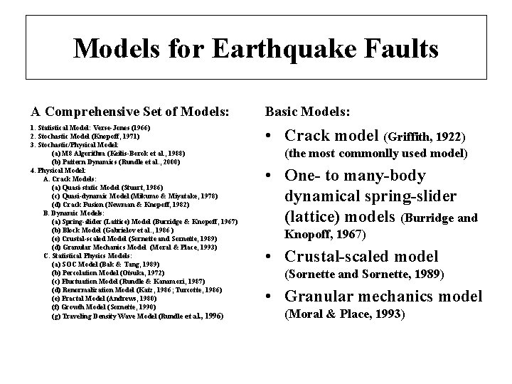
Models for Earthquake Faults A Comprehensive Set of Models: Basic Models: 1. Statistical Model: Verse-Jones (1966) 2. Stochastic Model (Knopoff, 1971) 3. Stochastic/Physical Model: (a) M 8 Algorithm (Keilis-Borok et al. , 1988) (b) Pattern Dynamics (Rundle et al. , 2000) 4. Physical Model: A. Crack Models: (a) Quasi-static Model (Stuart, 1986) (c) Quasi-dynamic Model (Mikumo & Miyatake, 1978) (d) Crack Fusion (Newman & Knopoff, 1982) B. Dynamic Models: (a) Spring-slider (Lattice) Model (Burridge & Knopoff, 1967) (b) Block Model (Gabrielov et al. , 1986 ) (e) Crustal-scaled Model (Sornette and Sornette, 1989) (d) Granular Mechanics Model (Moral & Place, 1993) C. Statistical Physics Models: (a) SOC Model (Bak & Tang, 1989) (b) Percolation Model (Otsuka, 1972) (c) Fluctuation Model (Rundle & Kanamori, 1987) (d) Renormalization Model (Katz, 1986; Turcotte, 1986) (e) Fractal Model (Andrews, 1980) (f) Growth Model (Sornette, 1990) (g) Traveling Density Wave Model (Rundle et al. , 1996) • Crack model (Griffith, 1922) (the most commonlly used model) • One- to many-body dynamical spring-slider (lattice) models (Burridge and Knopoff, 1967) • Crustal-scaled model (Sornette and Sornette, 1989) • Granular mechanics model (Moral & Place, 1993)

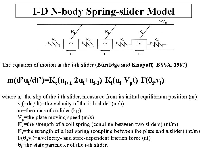
1 -D N-body Spring-slider Model The equation of motion at the i-th slider (Burridge and Knopoff, BSSA, 1967): m(d 2 ui/dt 2)=Kc(ui+1 -2 ui+ui-1)-Kl(ui-Vpt)-F(qi, vi) where ui=the slip of the i-th slider, measured from its initial equilibrium position (m) vi(=dui/dt)=the velocity of the i-th slider (m/s) m=the mass of a slider (kg) Vp=the plate moving speed (m/s) Kc=the strength of a coil spring (coupling between two sliders) (nt/m) Kl=the strength of a leaf spring (coupling between the plate and a slider) (nt/m) F(qi, vi)=a velocity- and state-dependent friction force (nt) qi=the state parameter of the i-th slider.

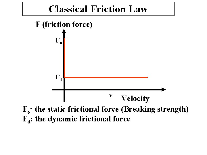
Classical Friction Law F (friction force) Fo Fd v Velocity Fo: the static frictional force (Breaking strength) Fd: the dynamic frictional force

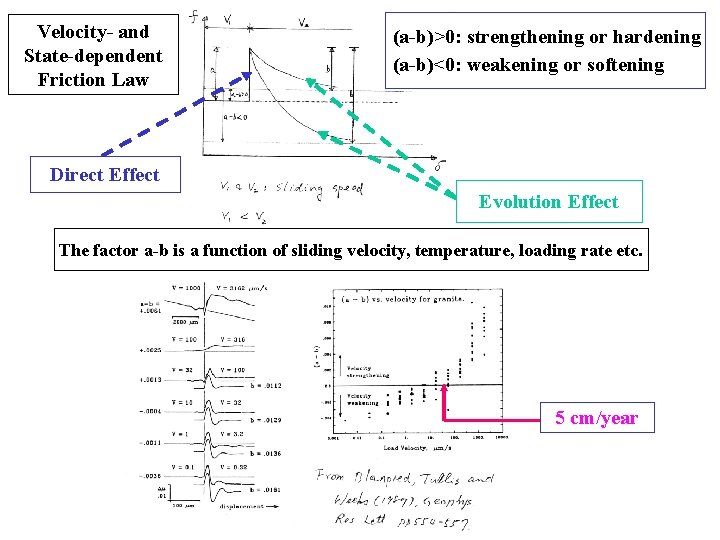
Velocity- and State-dependent Friction Law (a-b)>0: strengthening or hardening (a-b)<0: weakening or softening Direct Effect Evolution Effect The factor a-b is a function of sliding velocity, temperature, loading rate etc. 5 cm/year

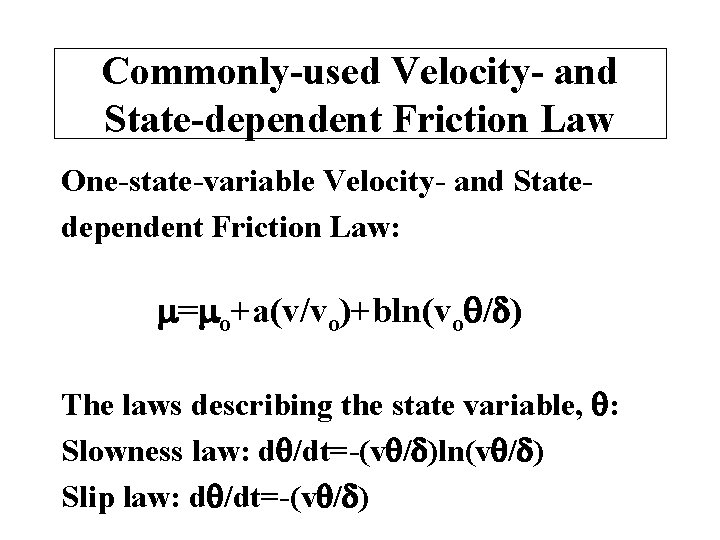
Commonly-used Velocity- and State-dependent Friction Law One-state-variable Velocity- and Statedependent Friction Law: = o+a(v/vo)+bln(voq/d) The laws describing the state variable, q: Slowness law: dq/dt=-(vq/d)ln(vq/d) Slip law: dq/dt=-(vq/d)

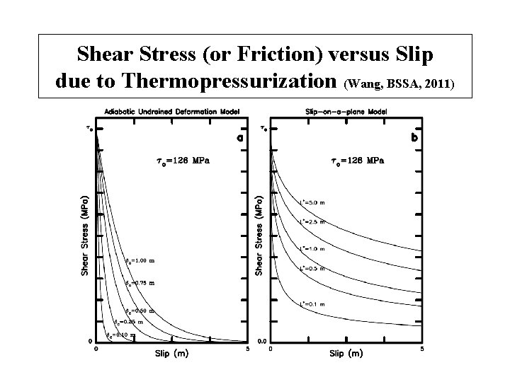
Shear Stress (or Friction) versus Slip due to Thermopressurization (Wang, BSSA, 2011)

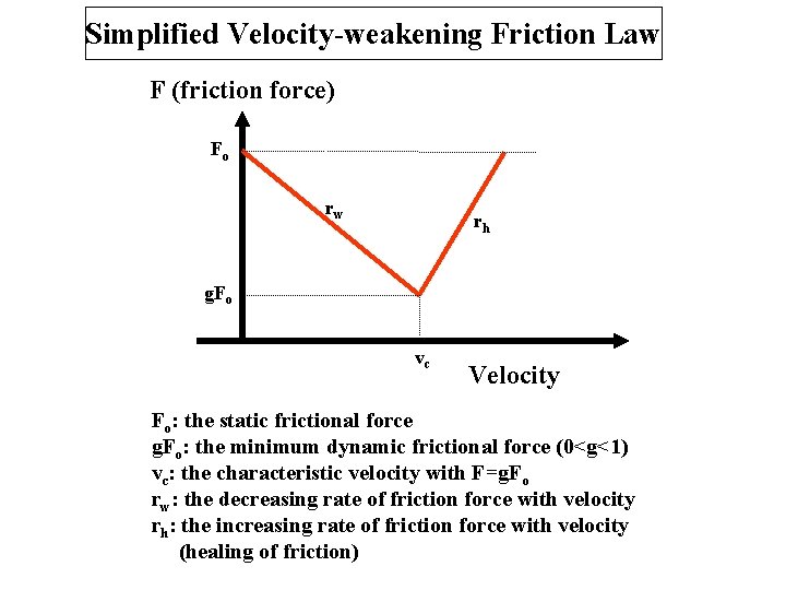
Simplified Velocity-weakening Friction Law F (friction force) Fo rw rh g. Fo vc Velocity Fo: the static frictional force g. Fo: the minimum dynamic frictional force (0<g<1) vc: the characteristic velocity with F=g. Fo rw: the decreasing rate of friction force with velocity rh: the increasing rate of friction force with velocity (healing of friction)

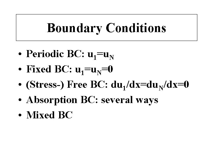
Boundary Conditions • • • Periodic BC: u 1=u. N Fixed BC: u 1=u. N=0 (Stress-) Free BC: du 1/dx=du. N/dx=0 Absorption BC: several ways Mixed BC

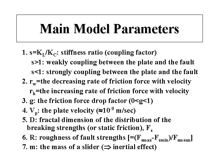
Main Model Parameters 1. s=KL/KC: stiffness ratio (coupling factor) s>1: weakly coupling between the plate and the fault s<1: strongly coupling between the plate and the fault 2. rw=the decreasing rate of friction force with velocity rh=the increasing rate of friction force with velocity 3. g: the friction force drop factor (0<g<1) 4. Vp: the plate velocity ( 10 -9 m/sec) 5. D: fractal dimension of the distribution of the breaking strengths (or static friction), Fs 6. R: roughness of fault strengths [=(Fsmax-Fsmin)/Fsmean] 7. m: the mass of a slider ( inertial effect)

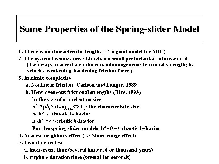
Some Properties of the Spring-slider Model 1. There is no characteristic length. (=> a good model for SOC) 2. The system becomes unstable when a small perturbation is introduced. (Two ways to arrest a rupture: a. inhomogeneous frictional strength; b. velocity-weakening-hardening friction force. ) 3. Intrinsic complexity a. Nonlinear friction (Carlson and Langer, 1989) b. Heterogeneous frictional strengths (Rice, 1993) h: the size of a nucleation size h*=2 dc/p(b-a)max Lc: the characteristic size h>h*=> chaotic behavior h<h* => periodic behavior For the spring-slider models, h*=0 => chaotic behavior 4. Nearest-neighbors effect (=> Short-range effect) 5. Two time scales: a. inter-event time (several hundred or thousand years) b. rupture duration time (several ten seconds)

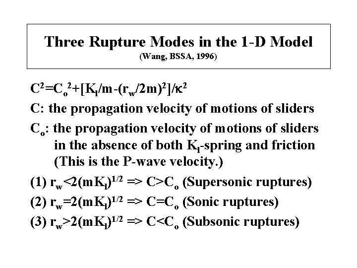
Three Rupture Modes in the 1 -D Model (Wang, BSSA, 1996) C 2=Co 2+[Kl/m-(rw/2 m)2]/k 2 C: the propagation velocity of motions of sliders Co: the propagation velocity of motions of sliders in the absence of both Kl-spring and friction (This is the P-wave velocity. ) (1) rw<2(m. Kl)1/2 => C>Co (Supersonic ruptures) (2) rw=2(m. Kl)1/2 => C=Co (Sonic ruptures) (3) rw>2(m. Kl)1/2 => C<Co (Subsonic ruptures)

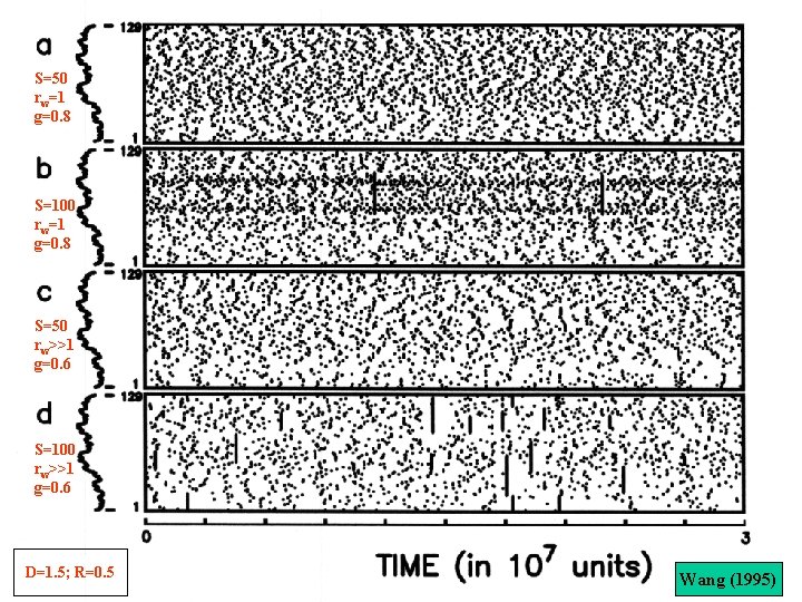
S=50 rw=1 g=0. 8 S=100 rw=1 g=0. 8 S=50 rw>>1 g=0. 6 S=100 rw>>1 g=0. 6 D=1. 5; R=0. 5 Wang (1995)

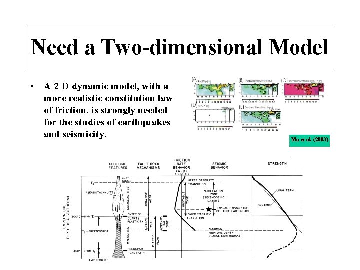
Need a Two-dimensional Model • A 2 -D dynamic model, with a more realistic constitution law of friction, is strongly needed for the studies of earthquakes and seismicity. Ma et al. (2003)

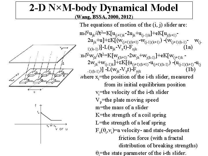
2 -D N×M-body Dynamical Model (Wang, BSSA, 2000, 2012) The equations of motion of the (i, j) slider are: m 2 ujk/ t 2=K[u(j+1)k-2 ujk+u(j-1)k]+e. K[uj(k+1)2 ujk+u]+e. K[(w(j+1)(k+1)-w(j-1)(k+1)) -(w(j+1)(k-1)- w(j(1 a) 1)(k-1))]-L(ujk-Vxt)-Fxjk m 2 wjk/ t 2=K[wj(k+1)-2 wjk+wj(k-1)]+e. K[w(j+1)k 2 wjk+w(j-1)k]+e. K[(u(j+1)(k+1)-u(j+1)(k-1)) -(u(j-1)(k+1)-u(j (1 b) -1)(k-1))] -L(wjk-Vyt)-Fyjk where xi=the position of the i-th slider, measured from its initial equilibrium position vi=the velocity of the i-th slider Vp=the plate moving speed m=the mass of a slider K=the strength of a coil spring L=the strength of a leaf spring Fo(qi, vi)=a velocity- and state-dependent friction force (with a fractal distribution of breaking strengths) q =the state parameter of the i-th slider.

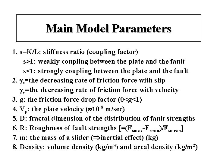
Main Model Parameters 1. s=K/L: stiffness ratio (coupling factor) s>1: weakly coupling between the plate and the fault s<1: strongly coupling between the plate and the fault 2. gs=the decreasing rate of friction force with slip gv=the decreasing rate of friction force with velocity 3. g: the friction force drop factor (0<g<1) 4. Vp: the plate velocity ( 10 -9 m/sec) 5. D: fractal dimension of the distribution of fault strengths 6. R: Roughness of fault strengths [=(Fsmax-Fsmin)/Fsmean] 7. m: the mass of a slider ( inertial effect) (kg) 8. Density: volume density (kg/m 3) and areal density (kg/m 2)

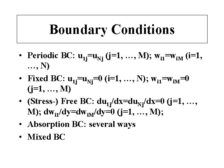
Boundary Conditions • Periodic BC: u 1 j=u. Nj (j=1, …, M); wi 1=wi. M (i=1, …, N) • Fixed BC: u 1 j=u. Nj=0 (i=1, …, N); wi 1=wi. M=0 (j=1, …, M) • (Stress-) Free BC: du 1 j/dx=du. Nj/dx=0 (j=1, …, M); dwi 1/dy=dwi. M/dy=0 (j=1, …, M); • Absorption BC: several ways • Mixed BC

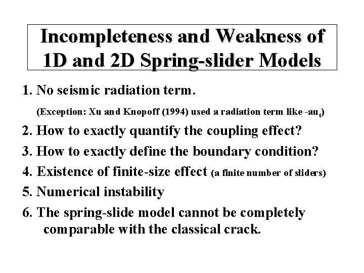
Incompleteness and Weakness of 1 D and 2 D Spring-slider Models 1. No seismic radiation term. (Exception: Xu and Knopoff (1994) used a radiation term like -aut) 2. How to exactly quantify the coupling effect? 3. How to exactly define the boundary condition? 4. Existence of finite-size effect (a finite number of sliders) 5. Numerical instability 6. The spring-slide model cannot be completely comparable with the classical crack.

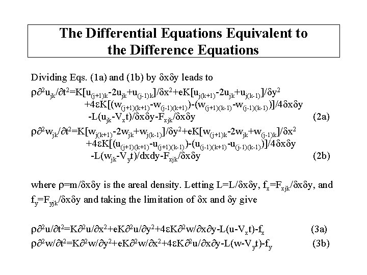
The Differential Equations Equivalent to the Difference Equations Dividing Eqs. (1 a) and (1 b) by dxdy leads to 2 ujk/ t 2=K[u(j+1)k-2 ujk+u(j-1)k]/dx 2+e. K[uj(k+1)-2 ujk+uj(k-1)]/dy 2 +4 e. K[(w(j+1)(k+1)-w(j-1)(k+1))-(w(j+1)(k-1)-w(j-1)(k-1))]/4 dxdy -L(ujk-Vxt)/dxdy-Fxjk/dxdy (2 a) 2 wjk/ t 2=K[wj(k+1)-2 wjk+wj(k-1)]/dy 2+e. K[w(j+1)k-2 wjk+w(j-1)k]/dx 2 +4 e. K[(u(j+1)(k+1)-u(j+1)(k-1))-(u(j-1)(k+1)-u(j-1)(k-1))]/4 dxdy -L(wjk-Vyt)/dxdy-Fxjk/dxdy (2 b) where =m/dxdy is the areal density. Letting L=L/dxdy, fx=Fxjk/dxdy, and fy=Fyjk/dxdy and taking the limitation of dx and dy give 2 u/ t 2=K 2 u/ x 2+e. K 2 u/ y 2+4 e. K 2 w/ x y-L(u-Vxt)-fx 2 w/ t 2=K 2 w/ y 2+e. K 2 w/ x 2+4 e. K 2 u/ x y-L(w-Vyt)-fy (3 a) (3 b)

General Forms of Solutions u(x, y, t)=u 1 e(ikr+Wt)+[Vxt-fx(0)]/L w(x, y, t)=w 1 e(ikr+Wt)+[Vyt-fy(0)]/L (4 a) (4 b) where k =<a, b>=vectorial wavenumber, w=angular frequency, and i=(-1)1/2. The scalar wavenumber is k=|k|. Inserting Eqs. (4 a) and (4 b) with r=<x, y> into Eqs. (3 a) and (3 b), respectively, leads to ( W 2+Ka 2+e. Kb 2+L-z. W)u 1+e. Kabw 1=0 e. Kabu 1+( W 2+Ka 2+e. Kb 2+L-z. W)w 1=0 (5 a) (5 b) Eqs. (5 a)–(5 b) => Mx=0, where M is a 2 2 matrix of the coefficients, x is a 2 1 matrix of u 1 and w 1, and 0 is the 2 1 zero matrix.

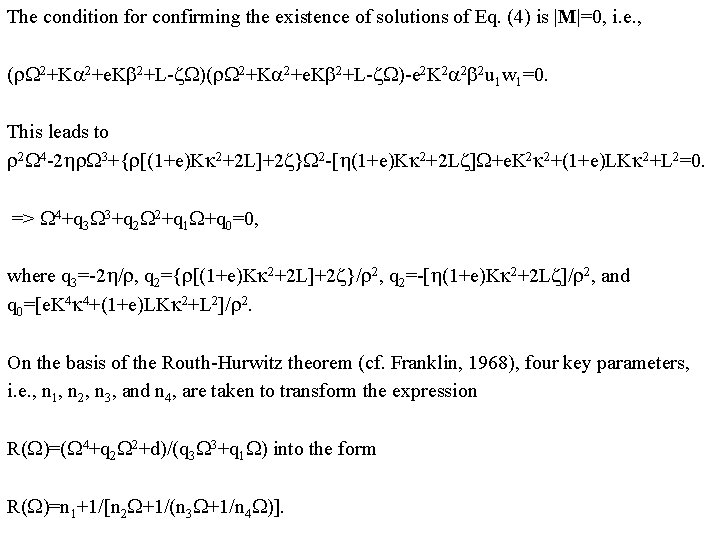
The condition for confirming the existence of solutions of Eq. (4) is |M|=0, i. e. , ( W 2+Ka 2+e. Kb 2+L-z. W)-e 2 K 2 a 2 b 2 u 1 w 1=0. This leads to 2 W 4 -2 h W 3+{ [(1+e)Kk 2+2 L]+2 z}W 2 -[h(1+e)Kk 2+2 Lz]W+e. K 2 k 2+(1+e)LKk 2+L 2=0. => W 4+q 3 W 3+q 2 W 2+q 1 W+q 0=0, where q 3=-2 h/ , q 2={ [(1+e)Kk 2+2 L]+2 z}/ 2, q 2=-[h(1+e)Kk 2+2 Lz]/ 2, and q 0=[e. K 4 k 4+(1+e)LKk 2+L 2]/ 2. On the basis of the Routh-Hurwitz theorem (cf. Franklin, 1968), four key parameters, i. e. , n 1, n 2, n 3, and n 4, are taken to transform the expression R(W)=(W 4+q 2 W 2+d)/(q 3 W 3+q 1 W) into the form R(W)=n 1+1/[n 2 W+1/(n 3 W+1/n 4 W)].

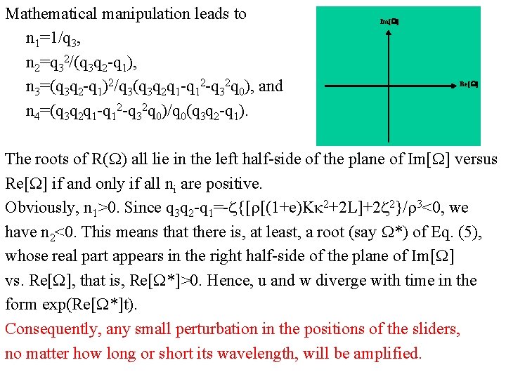
Mathematical manipulation leads to n 1=1/q 3, n 2=q 32/(q 3 q 2 -q 1), n 3=(q 3 q 2 -q 1)2/q 3(q 3 q 2 q 1 -q 12 -q 32 q 0), and n 4=(q 3 q 2 q 1 -q 12 -q 32 q 0)/q 0(q 3 q 2 -q 1). Im[W] Re[W] The roots of R(W) all lie in the left half-side of the plane of Im[W] versus Re[W] if and only if all ni are positive. Obviously, n 1>0. Since q 3 q 2 -q 1=-z{[ [(1+e)Kk 2+2 L]+2 z 2}/ 3<0, we have n 2<0. This means that there is, at least, a root (say W*) of Eq. (5), whose real part appears in the right half-side of the plane of Im[W] vs. Re[W], that is, Re[W*]>0. Hence, u and w diverge with time in the form exp(Re[W*]t). Consequently, any small perturbation in the positions of the sliders, no matter how long or short its wavelength, will be amplified.

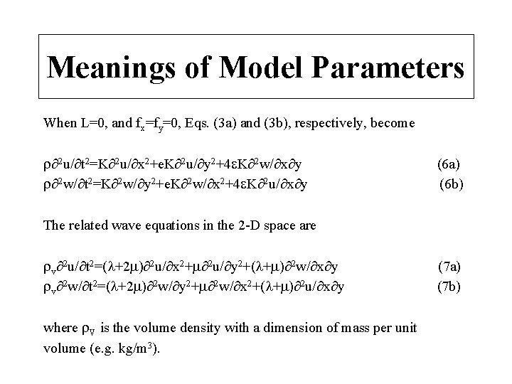
Meanings of Model Parameters When L=0, and fx=fy=0, Eqs. (3 a) and (3 b), respectively, become 2 u/ t 2=K 2 u/ x 2+e. K 2 u/ y 2+4 e. K 2 w/ x y 2 w/ t 2=K 2 w/ y 2+e. K 2 w/ x 2+4 e. K 2 u/ x y (6 a) (6 b) The related wave equations in the 2 -D space are v 2 u/ t 2=( +2 ) 2 u/ x 2+ 2 u/ y 2+( + ) 2 w/ x y v 2 w/ t 2=( +2 ) 2 w/ y 2+ 2 w/ x 2+( + ) 2 u/ x y where V is the volume density with a dimension of mass per unit volume (e. g. kg/m 3). (7 a) (7 b)

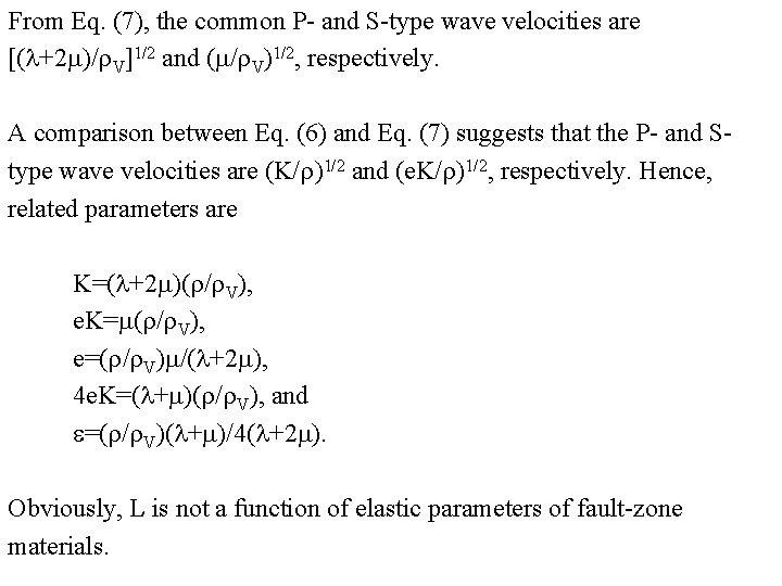
From Eq. (7), the common P- and S-type wave velocities are [( +2 )/ V]1/2 and ( / V)1/2, respectively. A comparison between Eq. (6) and Eq. (7) suggests that the P- and Stype wave velocities are (K/ )1/2 and (e. K/ )1/2, respectively. Hence, related parameters are K=( +2 )( / V), e. K= ( / V), e=( / V) /( +2 ), 4 e. K=( + )( / V), and e=( / V)( + )/4( +2 ). Obviously, L is not a function of elastic parameters of fault-zone materials.

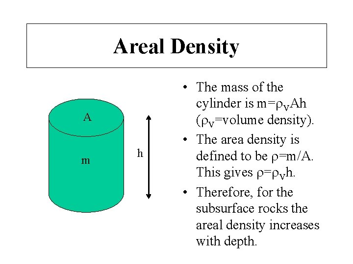
Areal Density A m h • The mass of the cylinder is m= VAh ( V=volume density). • The area density is defined to be =m/A. This gives = Vh. • Therefore, for the subsurface rocks the areal density increases with depth.

How to evaluate L?

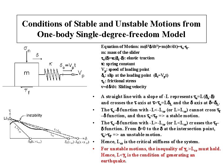
Conditions of Stable and Unstable Motions from One-body Single-degree-freedom Model Equation of Motion: m(d 2 d/dt 2)=m(dv/dt)=te-tf. m: mass of the slider te(d)=k(do-d): elastic traction k: spring constant Vp: speed of loading point do: slip at the loading point (do=Vpt) tf : frictional stress v=dd/dt: Sliding velocity • • • A straight line with a slope of -L represents te=L(do-d) and crosses the t axis at t=to=Ld. L and the d axis at d=d. L. The te–d function with -L<-Lcr (or L>Lcr) cannot cross tf –d function, and thus te<tf. => a stable motion. The te–d function with -L>-Lcr (or L<Lcr) crosses the tf– d function. From d=0 to the d at the intersection point, te>tf. => an unstable motion. Hence, Lcr is the critical stiffness of the system. For unstable motions, the inequality of gs >Lcr must hold. Hence, L<gs is the condition of generating an earthquake.

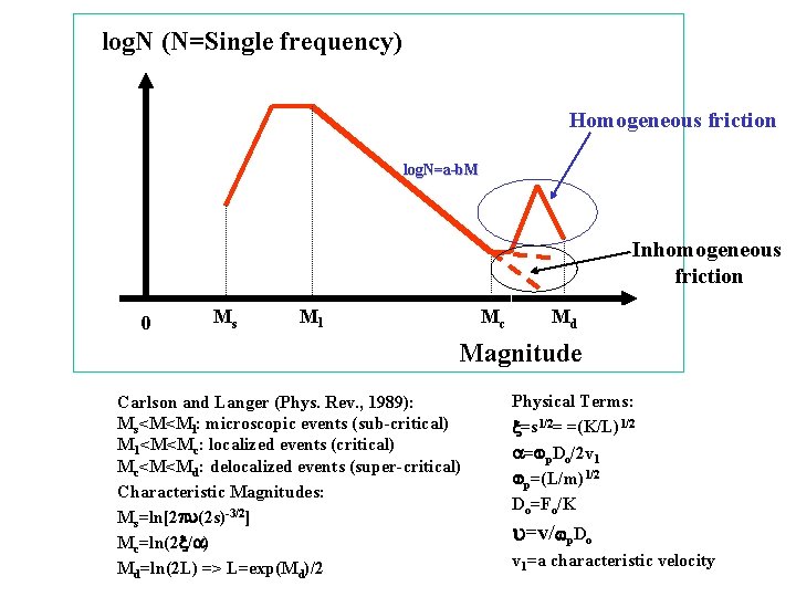
log. N (N=Single frequency) Homogeneous friction log. N=a-b. M Inhomogeneous friction 0 Ms Ml Mc Md Magnitude Carlson and Langer (Phys. Rev. , 1989): Ms<M<Ml: microscopic events (sub-critical) M 1<M<Mc: localized events (critical) Mc<M<Md: delocalized events (super-critical) Characteristic Magnitudes: Ms=ln[2 pu(2 s)-3/2] Mc=ln(2 x/a) Md=ln(2 L) => L=exp(Md)/2 Physical Terms: x=s 1/2= =(K/L)1/2 a=wp. Do/2 v 1 wp=(L/m)1/2 Do=Fo/K u=v/wp. Do v 1=a characteristic velocity

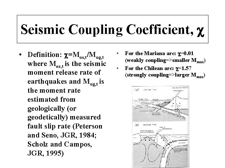
Seismic Coupling Coefficient, c • Definition: c=Mos, t/Mog, t where Mos, t is the seismic moment release rate of earthquakes and Mog, t is the moment rate estimated from geologically (or geodetically) measured fault slip rate (Peterson and Seno, JGR, 1984; Scholz and Campos, JGR, 1995) • • For the Mariana arc: c=0. 01 (weakly coupling=>smaller Mmax) For the Chilean arc: c=1. 57 (strongly coupling=>larger Mmax)

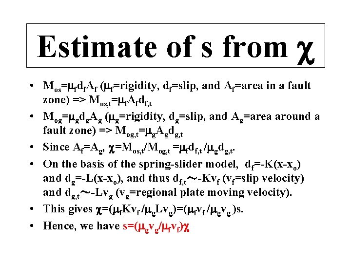
Estimate of s from c • Mos= fdf. Af ( f=rigidity, df=slip, and Af=area in a fault zone) => Mos, t= f. Afdf, t • Mog= gdg. Ag ( g=rigidity, dg=slip, and Ag=area around a fault zone) => Mog, t= g. Agdg, t • Since Af=Ag, c=Mos, t/Mog, t = fdf, t / gdg, t. • On the basis of the spring-slider model, df=-K(x-xo) and dg=-L(x-xo), and thus df, t～-Kvf (vf=slip velocity) and dg, t～-Lvg (vg=regional plate moving velocity). • This gives c=( f. Kvf / g. Lvg)=( fvf / gvg )s. • Hence, we have s=( gvg/ fvf)c

Angular Frequency and Phase Velocity The trial solutions are u~exp[i(kr-wt)] along the x-axis and w~exp[i(krwt)] along the y-axis. Since k=<a, b> and r=<x, y>, we have u~exp[i(ax+by-wt)] and w~exp[i(ax+by-wt)]. Inserting Eq. (6) the trial solutions results in ( w 2 -Ka 2 -e. Kb 2)u-4 e. Kabw=0 -4 e. Kabu+( w 2 -Kb 2 -e. Ka 2)w=0 (8 a) (8 b) Eq. (8) => Mu=0, where M is a 2 2 matrix of coefficients and u is a 2 1 matrix of u and w.

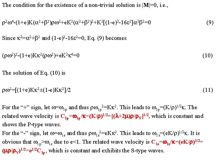
The condition for the existence of a non-trivial solution is |M|=0, i. e. , 2 w 4 -(1+e)K(a 2+b 2) w 2+e. K 2(a 2+b 2)2+K 2[(1 -e)2 -16 e 2]a 2 b 2=0 (9) Since k 2=a 2+b 2 and (1 -e)2 -16 e 2=0, Eq. (9) becomes ( w 2)2 -(1+e)Kk 2( w 2)+e. K 2 k 4=0 (10) The solution of Eq. (10) is w 2=[(1+e)Kk 2±(1 -e)Kk 2]/2 (11) For the “+” sign, let w=w 1 p and thus w 1 p 2=Kk 2. This leads to w 1 p=(K/ )1/2 k. The related wave velocity is C 1 p=w 1 p/k=(K/ )1/2=[( +2 ) / V]1/2, which is constant and shows the P-type waves. For the “-” sign, let w=w 1 s and thus w 1 s 2=e. Kk 2. This leads to w 1 s=(e. K/ )1/2 k. It is obvious that w 1 p>w 1 s due to e<1. The related wave velocity is C 1 s=w 1 s/k=(e. K/ )1/2= ( / V)1/2=e 1/2 C 1 p, which is constant and exhibits the S-type waves.

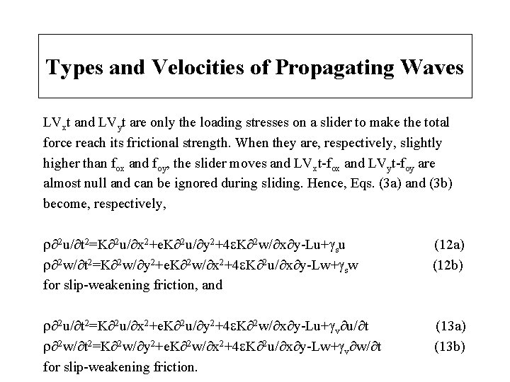
Types and Velocities of Propagating Waves LVxt and LVyt are only the loading stresses on a slider to make the total force reach its frictional strength. When they are, respectively, slightly higher than fox and foy, the slider moves and LVxt-fox and LVyt-foy are almost null and can be ignored during sliding. Hence, Eqs. (3 a) and (3 b) become, respectively, 2 u/ t 2=K 2 u/ x 2+e. K 2 u/ y 2+4 e. K 2 w/ x y-Lu+gsu 2 w/ t 2=K 2 w/ y 2+e. K 2 w/ x 2+4 e. K 2 u/ x y-Lw+gsw for slip-weakening friction, and (12 a) (12 b) 2 u/ t 2=K 2 u/ x 2+e. K 2 u/ y 2+4 e. K 2 w/ x y-Lu+gv u/ t 2 w/ t 2=K 2 w/ y 2+e. K 2 w/ x 2+4 e. K 2 u/ x y-Lw+gv w/ t for slip-weakening friction. (13 a) (13 b)

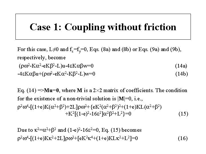
Case 1: Coupling without friction For this case, L≠ 0 and fx=fy=0, Eqs. (8 a) and (8 b) or Eqs. (9 a) and (9 b), respectively, become ( w 2 -Ka 2 -e. Kb 2 -L)u-4 e. Kabw=0 (14 a) -4 e. Kabu+( w 2 -e. Ka 2 -Kb 2 -L)w=0 (14 b) Eq. (14) =>Mu=0, where M is a 2 2 matrix of coefficients. The condition for the existence of a non-trivial solution is |M|=0, i. e. , 2 w 4 -[(1+e)K(a 2+b 2)+2 L] w 2+{e. K 2(a 2+b 2)2+(1+e)KL(a 2+b 2) +K 2[(1 -e)2 -16 e 2]a 2 b 2+L 2}=0 (15) Due to k 2=a 2+b 2 and (1 -e)2 -16 e 2=0, Eq. (15) becomes 2 w 4 -[(1+e)Kk 2+2 L] w 2+[e. K 2 k 4+(1+e)KLk 2+L 2]=0 (16)

The solution of Eq. (16) is w 2={[(1+e)±(1 -e)]Kk+2 L}/2. Remarkably, coupling results in a constant increase in angular frequency and thus behaves like a low-cut filter. The related wave velocity, C, is C 2=(w/k)2={[(1+e)±(1 -e)](K/ )+2 L/ k 2}/2. For the “+” sign, let C=C 2 p and thus C 2 p=(C 1 p 2+L/ k 2)1/2 (17) The additional amount of wave velocity decreases with increasing k. When k>>1, C 2 p≈C 1 p. For finite k, C 2 p>C 1 p. Thus, this inequality and k-dependence of C 2 p show supersonic, dispersed P-type waves. When L=0, C 2 p=C 1 p. For the “-” sign, let C=C 2 s and thus C 2 s=(C 1 s 2+L/ k 2)1/2 The additional amount of wave velocity decreases with increasing k. When k>>1, C 2 s≈C 1 s. For finite k, C 2 s>C 1 s. Thus, this inequality and k-dependence of C 2 s show supershear, dispersed S-type waves. When L=0, C 2 s=C 1 s. (18)

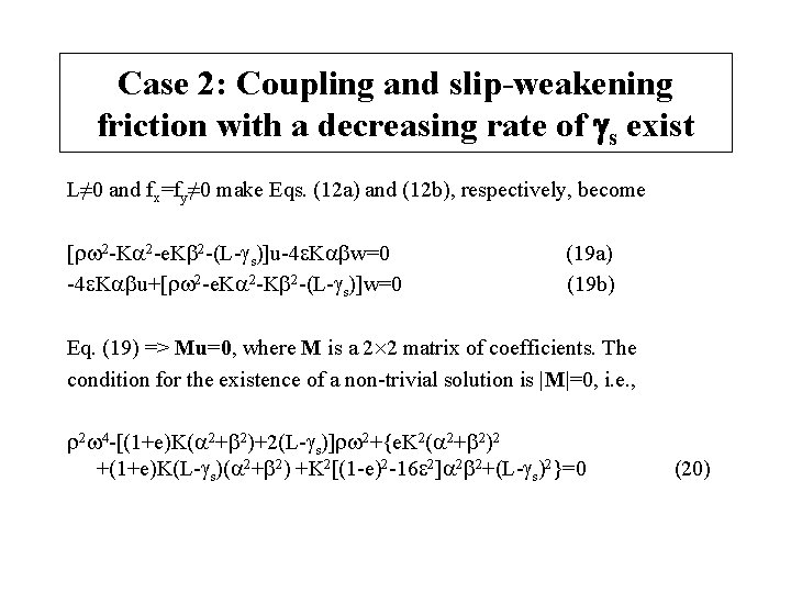
Case 2: Coupling and slip-weakening friction with a decreasing rate of gs exist L≠ 0 and fx=fy≠ 0 make Eqs. (12 a) and (12 b), respectively, become [ w 2 -Ka 2 -e. Kb 2 -(L-gs)]u-4 e. Kabw=0 -4 e. Kabu+[ w 2 -e. Ka 2 -Kb 2 -(L-gs)]w=0 (19 a) (19 b) Eq. (19) => Mu=0, where M is a 2 2 matrix of coefficients. The condition for the existence of a non-trivial solution is |M|=0, i. e. , 2 w 4 -[(1+e)K(a 2+b 2)+2(L-gs)] w 2+{e. K 2(a 2+b 2)2 +(1+e)K(L-gs)(a 2+b 2) +K 2[(1 -e)2 -16 e 2]a 2 b 2+(L-gs)2}=0 (20)

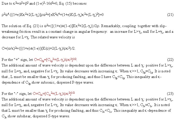
Due to k 2=a 2+b 2 and (1 -e)2 -16 e 2=0, Eq. (15) becomes 2 w 4 -[(1+e)Kk 2+2(L-gs)] w 2+[e. K 2 k 4+(1+e)K(L-gs)k 2+(L-gs)2]=0 (21) The solution of Eq. (21) is w 2={[(1+e)±(1 -e)]Kk 2+2(L-gs)}/2. Remarkably, coupling together with slipweakening friction result in a constant change in angular frequency: an increase for L>gs, null for L=gs, and a decrease for L<gs. The related wave velocity is C=(w/k)2={[(1+e)±(1 -e)](K/ )+2(L-gs)/ k 2}/2. For the “+” sign, let C=C 3 p=[C 1 p 2+(L-gs)/ k 2]1/2. (22) The additional amount of wave velocity is dependent upon the difference between L and gs: positive for L>gs, null for L=gs, and, negative for L<gs. Its value decreases with increasing k. When k>>1, C 3 p≈C 1 p. It is noted that , L must be smaller than gs for producing faulting, and thus I have C 3 p<C 1 p. This inequality and kdependence of C 3 p show subsonic, dispersed P-type waves. For the "-" sign, let C=C 3 s=[C 1 s 2+(L-gs)/ k 2]1/2 (23) The additional amount of wave velocity is dependent upon the difference between L and gs: positive for L>gs, null for L=gs, and, negative for L<gs. Its value decreases with increasing k. When k>>1, C 3 s≈C 1 s. It is noted that L must be smaller than gs for producing faulting, and thus C 3 s<C 1 s. This inequality and k-dependence of C 3 s show subshear, dispersed S-type waves.

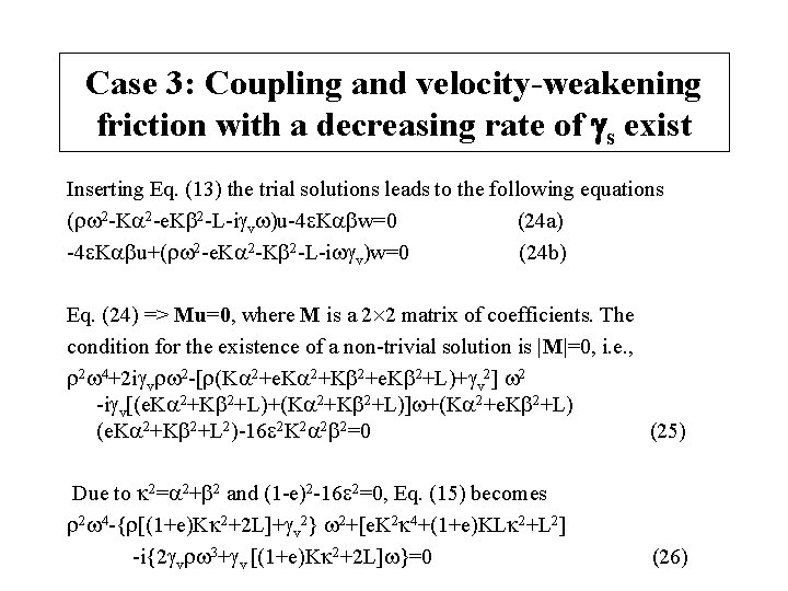
Case 3: Coupling and velocity-weakening friction with a decreasing rate of gs exist Inserting Eq. (13) the trial solutions leads to the following equations ( w 2 -Ka 2 -e. Kb 2 -L-igvw)u-4 e. Kabw=0 (24 a) -4 e. Kabu+( w 2 -e. Ka 2 -Kb 2 -L-iwgv)w=0 (24 b) Eq. (24) => Mu=0, where M is a 2 2 matrix of coefficients. The condition for the existence of a non-trivial solution is |M|=0, i. e. , 2 w 4+2 igv w 2 -[ (Ka 2+e. Ka 2+Kb 2+e. Kb 2+L)+gv 2] w 2 -igv[(e. Ka 2+Kb 2+L)+(Ka 2+Kb 2+L)]w+(Ka 2+e. Kb 2+L) (e. Ka 2+Kb 2+L 2)-16 e 2 K 2 a 2 b 2=0 (25) Due to k 2=a 2+b 2 and (1 -e)2 -16 e 2=0, Eq. (15) becomes 2 w 4 -{ [(1+e)Kk 2+2 L]+gv 2} w 2+[e. K 2 k 4+(1+e)KLk 2+L 2] -i{2 gv w 3+gv [(1+e)Kk 2+2 L]w}=0 (26)

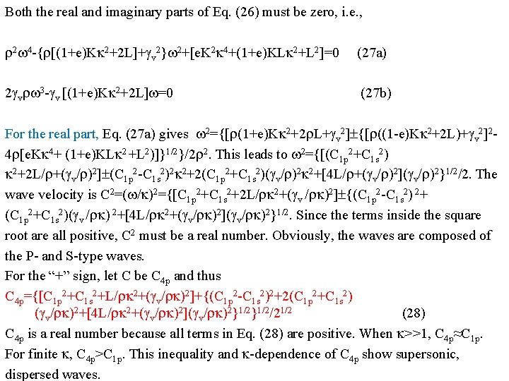
Both the real and imaginary parts of Eq. (26) must be zero, i. e. , 2 w 4 -{ [(1+e)Kk 2+2 L]+gv 2}w 2+[e. K 2 k 4+(1+e)KLk 2+L 2]=0 (27 a) 2 gv w 3 -gv [(1+e)Kk 2+2 L]w=0 (27 b) For the real part, Eq. (27 a) gives w 2={[ (1+e)Kk 2+2 L+gv 2] {[ ((1 -e)Kk 2+2 L)+gv 2]24 [e. Kk 4+ (1+e)KLk 2+L 2)]}1/2}/2 2. This leads to w 2={[(C 1 p 2+C 1 s 2) k 2+2 L/ +(gv/ )2] (C 1 p 2 -C 1 s 2)2 k 2+2(C 1 p 2+C 1 s 2)(gv/ )2 k 2+[4 L/ +(gv/ )2](gv/ )2}1/2/2. The wave velocity is C 2=(w/k)2={[C 1 p 2+C 1 s 2+2 L/ k 2+(gv / k)2] {(C 1 p 2 -C 1 s 2) 2+ (C 1 p 2+C 1 s 2)(gv / k) 2+[4 L/ k 2+(gv/ k)2](gv/ k)2}1/2. Since the terms inside the square root are all positive, C 2 must be a real number. Obviously, the waves are composed of the P- and S-type waves. For the “+” sign, let C be C 4 p and thus C 4 p={[C 1 p 2+C 1 s 2+L/ k 2+(gv/ k)2]+{(C 1 p 2 -C 1 s 2)2+2(C 1 p 2+C 1 s 2) (gv/ k)2+[4 L/ k 2+(gv/ k)2](gv/ k)2}1/2/21/2 (28) C 4 p is a real number because all terms in Eq. (28) are positive. When k>>1, C 4 p≈C 1 p. For finite k, C 4 p>C 1 p. This inequality and k-dependence of C 4 p show supersonic, dispersed waves.

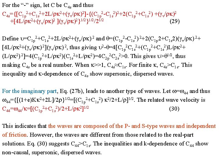
For the “-” sign, let C be C 4 s and thus C 4 s={[C 1 p 2+C 1 s 2+2 L/ k 2+(gv/ k)2]-{(C 1 p 2 -C 1 s 2)2+2(C 1 p 2+C 1 s 2) +(gv/ k)2 +[4 L/ k 2+(gv/ k)2 ](gv/ k)2}1/2/21/2 (29) Define u=C 1 p 2+C 1 s 2+2 L/ k 2+(gv/ k) 2 and q=(C 1 p 2 -C 1 s 2) 2+2(C 1 p 2+C 1 s 2)(gv/ k) 2+ [4 L/ k 2+(gv/ k) 2](gv/ k) 2, thus giving u 2 -q=4[C 1 p 2 C 1 s 2+(C 1 p 2+C 1 s 2)L/ k 2+ (L/ k 2) 2]=4(C 1 p 2+L/ k 2)(C 1 s 2+L/ k 2)=4 C 2 p 2 C 2 s 2>0. This gives u>q 1/2, thus making C 4 s be a real number. When k>>1, C 4 s≈C 1 s. For finite k, C 4 s>C 1 s. This inequality and k-dependence of C 4 s show supersonic, dispersed waves. For the imaginary part, Eq. (27 b), leads to another type of waves. Let w=w 44 and thus w 44={[(1+e)Kk 2+2 L]/2 }1/2=[(C 1 p 2+C 1 s 2) k 2/2+L/ ]1/2. The related wave velocity is C 44=w 44/k=[(C 1 p 2+C 1 s 2)/2+L/ k 2]1/2 (30) This indicates that the waves are composed of the P- and S-type waves and independent of friction. However, the waves are different from those related to the real-part solutions. Eq. (30) suggests C 44>C 1 s. The inequalities and k-dependence of C 44 show non-causal, supersonic, dispersed waves.

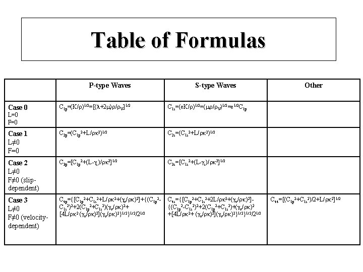
Table of Formulas P-type Waves S-type Waves C 1 p=(K/ )1/2=[( +2 ) / V]1/2 C 1 s=(e. K/ )1/2=( / V)1/2=e 1/2 C 1 p Case 1 L≠ 0 F=0 C 2 p=(C 1 p 2+L/ k 2)1/2 C 2 s=(C 1 s 2+L/ k 2)1/2 Case 2 L≠ 0 F≠ 0 (slipdependent) C 3 p=[C 1 p 2+(L-gs)/ k 2]1/2 C 3 s=[C 1 s 2+(L-gs)/ k 2]1/2 Case 3 L≠ 0 F≠ 0 (velocitydependent) C 4 p={[C 1 p 2+C 1 s 2+L/ k 2+(gv/ k)2]+{(C 1 p 2 C 1 s 2)2+2(C 1 p 2+C 1 s 2)(gv/ k)2+ [4 L/ k 2 (gv/ k)2](gv/ k)2}1/2/21/2 C 4 s={[C 1 p 2+C 1 s 2+2 L/ k 2+(gv/ k)2]{(C 1 p 2 -C 1 s 2)2+2(C 1 p 2+C 1 s 2)+(gv/ k)2 +[4 L/ k 2+ (gv/ k)2](gv/ k)2}1/2/21/2 Case 0 Other L=0 F=0 C 44=[(C 1 p 2+C 1 s 2)/2+L/ k 2]1/2

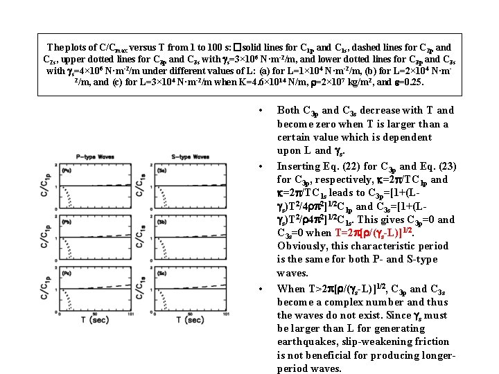
The plots of C/Cmax versus T from 1 to 100 s: �solid lines for C 1 p and C 1 s, dashed lines for C 2 p and C 2 s, upper dotted lines for C 3 p and C 3 s with gs=3× 106 N·m-2/m, and lower dotted lines for C 3 p and C 3 s with gs=4× 106 N·m-2/m under different values of L: (a) for L=1× 104 N·m-2/m, (b) for L=2× 104 N·m 2/m, and (c) for L=3× 104 N·m-2/m when K=4. 6× 1014 N/m, =2× 107 kg/m 2, and e=0. 25. • • • Both C 3 p and C 3 s decrease with T and become zero when T is larger than a certain value which is dependent upon L and gs. Inserting Eq. (22) for C 3 p and Eq. (23) for C 3 p, respectively, k=2 p/TC 1 p and k=2 p/TC 1 s leads to C 3 p=[1+(Lgs)T 2/4 p 2]1/2 C 1 p and C 3 s=[1+(Lgs)T 2/ 4 p 2]1/2 C 1 s. This gives C 3 p=0 and C 3 s=0 when T=2 p[ /(gs-L)]1/2. Obviously, this characteristic period is the same for both P- and S-type waves. When T>2 p[ /(gs-L)]1/2, C 3 p and C 3 s become a complex number and thus the waves do not exist. Since gs must be larger than L for generating earthquakes, slip-weakening friction is not beneficial for producing longerperiod waves.

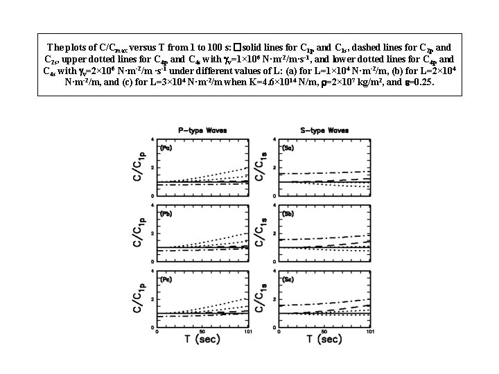
The plots of C/Cmax versus T from 1 to 100 s: �solid lines for C 1 p and C 1 s, dashed lines for C 2 p and C 2 s, upper dotted lines for C 4 p and C 4 s with gv=1× 106 N·m-2/m·s-1, and lower dotted lines for C 4 p and C 4 s with gv=2× 106 N·m-2/m ·s-1 under different values of L: (a) for L=1× 104 N·m-2/m, (b) for L=2× 104 N·m-2/m, and (c) for L=3× 104 N·m-2/m when K=4. 6× 1014 N/m, =2× 107 kg/m 2, and e=0. 25.

Summary • • • There are only two types of waves for Cases 0, 1, and 2: One is the P-type wave and the other the S-type wave. For Case 3, there are three types of waves, which are all composed of the P- and Stype waves. However, the first and second types of waves are, respectively, similar to the P- and S-type waves. The velocity of the third type of waves is always lower than the P-type wave velocity and higher than the S-type wave velocity. In other words, there are the subrsonic and supershear waves. Coupling (for Cases 2 and 3) clearly increases the velocities of the two types of waves, thus leading to supersonic and supershear waves. Slip-weakening friction for Case 2 decreases the velocities, thus only being able to result in subsonic and subshear waves. When the period T>2 p[ /(gs-L)]1/2, the waves do not exist for slip-decreasing friction, because gs must be larger than L for generating earthquakes. Hence, slipweakening friction is not beneficial for producing longer-period waves. Velocity-weakening friction makes the velocities of the first type of waves higher than the P-type wave velocity, while it makes the velocity of the second type of waves higher or lower than the S-type wave velocity just depending on the combination of L and gv.

謝謝 (Thanks)