Dynamical Models of Decision Making Optimality human performance

Dynamical Models of Decision Making Optimality, human performance, and principles of neural information processing Jay Mc. Clelland Department of Psychology and Center for Mind Brain and Computation Stanford University

Is the rectangle longer toward the northwest or longer toward the northeast?

2. 00 ” Longer toward the Northeast! 1. 99 ”

An Abstract Statistical Theory • How do you decide if an urn contains more black balls or white balls? – We assume you can only draw balls one at a time and want to stop as soon as you have enough evidence to achieve a desired level of accuracy. – You know in advance that the proportion of black balls is either p or 1 -p.

Optimal Policy (Sequential Probability Ratio Test) • Reach in and grab a ball. • Keep track of difference = #black - #white. • A given difference n occurs with probability pn/(1 -p)n – E. g. , if p is either. 9 or. 1: • With n = 1, we’ll be right 9 times out of 10 if we say “black” • With n = 2, we’ll be right 81 times out of 82 if we say “black” • So, respond when the difference n reaches a criterion value +C or -C, set based on p to produce a desired level of accuracy. • This policy produces fastest possible decisions on average for a given level of accuracy.

The Drift Diffusion Model • Continuous version of the SPRT • A random decision variable x is initialized at 0. • At each time step a small random step is taken. • Mean direction of steps is +m for one alternative, –m for the other. • Size of m corresponds to discriminability of the alternatives. • Start at 0, respond when criterion is reached. • Alternatively, in ‘time controlled’ tasks, respond when a response signal is given.

Two Problems with the DDM Accuracy should gradually improve toward 100% correct, even for very hard discriminations, as stimulus processing time is allowed to increase, but this is not what is observed in data. • The model also predicts both correct and incorrect RT’s will be equally fast for a given level of difficulty, but incorrect RT’s are generally slower than correct RT’s. • These findings present problems for models based on DDM/SPRT in both the psychological and neuroscience literature (e. g. , Mazurek et al, 2003). Hard Errors RT • Prob. Correct Easy Correct Responses Hard -> Easy

Goals of Our Research • We seek an understanding of how dynamical neural processes in the brain give rise the patterns of behavior seen in decision making situations. • We seek a level of analysis in describing the neural processes that can be linked to behavior on the one hand the details of neural processes on the other. • We seek to understand individual differences in processing and the brain basis of these differences. • Future direction: Can processing dynamics be optimized by training?

Usher and Mc. Clelland (2001) Leaky Competing Accumulator Model • Addresses the process of deciding between two alternatives based neural population variables subject to external input (. 5 +/-m/2) with leakage, self-excitation, mutual inhibition, and noise: dx 1/dt =. 5+m/2 -l(x 1)+af(x 1)–bf(x 2)+x 1 dx 2/dt =. 5 -m/2 -l(x 2)+af(x 2)–bf(x 1)+x 2 • The difference x 1 – x 2 reduces to the DDM under certain conditions, but produces a range of interesting features under other conditions. + - +

Dynamics of winning and loosing populations in the brain and the LCAM

Wong & Wang (2006) ~Usher & Mc. Clelland (2001)

Usher and Mc. Clelland (2001) Leaky Competing Accumulator Model • Addresses the process of deciding between two alternatives based neural population variables subject to external input (. 5 +/-m/2) with leakage, self-excitation, mutual inhibition, and noise: dx 1/dt =. 5+m/2 -l(x 1)+af(x 1)–bf(x 2)+x 1 dx 2/dt =. 5 -m/2 -l(x 2)+af(x 2)–bf(x 1)+x 2 • How does the model behave as a function of different choices of parameters? + - +

Roles of (k = l–a) and b

Time-accuracy curves for different |k -b| |k-b| = 0 |k-b| =. 2 |k-b| =. 4

Testing the model • Quantitative tests: – Detailed fits to various aspects of experimental data, including shapes of ‘time-accuracy curves’ • Qualitative test: – Understanding the dynamics of the model leads to a novel prediction

* *OU = analytic approx to LCAM; DDV = DDM w/ between trial drift variance (Ratcliff, 1978)

Assessing Integration Dynamics • • Participant sees stream of S’s and H’s Must decide which is predominant 50% of trials last ~500 msec, allow accuracy assessment 50% are ~250 msec, allow assessment of dynamics – These streams contain an equal # of S’s and H’s But there are clusters bunched together at the end (0, 2 or 4). Leak-dominant Inhibition-dominant Favored early Favored late

• Large individual differences. • Subjects show both kinds of biases. • The less the bias, the higher the accuracy, as predicted. S 3

Extension to N alternatives • Extension to n alternatives is very natural. • Model accounts quite well for Hick’s law (RT increases with log n alternatives), assuming that threshold is raised with n to maintain equal accuracy in all conditions. • Use of non-linear activation function increases efficiency when there are only a few alternatives ‘in contention’ given the stimulus.

Integration of reward and motion information (Rorie & Newsome) Monkey’s choices reflect a beautifully regular combination of the effects of stimulus coherence and reward. Bias is slightly sub-optimal.

Population response of LIP Neurons in two reward conditions Choose in Choose out

Some Open Questions • How localized vs. distributed are the neural populations involved in decisions? • What does it mean in the brain to pass the threshold for response initiation? • Are dynamics of reward biases tuned to allow a practiced participant to optimize decisions, combining reward and stimulus information in the right mix to achieve (near) optimality?

Human Experiment Examining Reward Bias Effect at Different Time Points after Target Onset • Target stimuli are rectangles shifted 1, 3, or 5 pixels L or R of fixation • Reward cue occurs 750 msec before stimulus. – – • Small arrow head pointing L or R visible for 250 msec. Only biased reward conditions (2 vs 1 and 1 vs 2) are used. Response signal occurs at different times after target onset: 0 75 150 225 300 450 600 900 1200 2000 - Participant receives reward only if response is correct and occurs within 250 msec of response signal. - Participants were run for 15 -25 sessions to provide stable data. - Data shown are from later sessions in which effects were all stable.

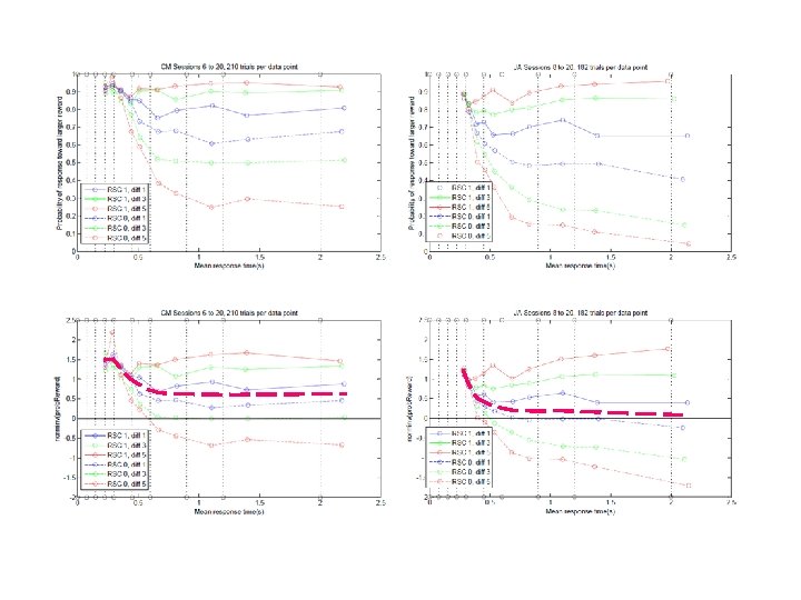
A participant with very little reward bias • Top panel shows probability of response giving larger reward as a function of actual response time for combinations of: Stimulus shift (1 3 5) pixels Reward-stimulus compatibility • Lower panel shows data transformed to z scores, and corresponds to theoretical construct: mean(x 1(t)-x 2(t))+bias(t) sd(x 1(t)-x 2(t)) where x 1 represents the state of the accumulator associated with greater reward, x 2 the same for lesser reward, and S is thought to choose larger reward if x 1(t)-x 2(t)+bias(t) > 0.

Participants Showing Reward Bias

Possible Models • Data are not consistent with bias as initial input that decays exponentially (except for possibly 1 participant). • Nor are data consistent with treating the bias as an additional constant input. • Instead it appears that bias starts large and falls to a fixed residual, as would be appropriate for optimal performance. • Bias is not large enough to achieve maximal reward rate, however.

Some Take-Home Messages and a Question • Participants vary in details of brain dynamics of both stimulus and reward processing. • Some are capable of achieving far closer approximations to optimality than others. • Participants generally appear more concerned with being right than with maximizing reward outcomes. • Question: – Can we train optimization of the dynamics of decision making?