Dynamic Time Warping Algorithm Slides from Elena Tsiporkova

Dynamic Time Warping Algorithm Slides from: Elena Tsiporkova

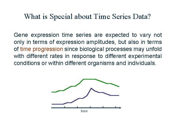
What is Special about Time Series Data? Gene expression time series are expected to vary not only in terms of expression amplitudes, but also in terms of time progression since biological processes may unfold with different rates in response to different experimental conditions or within different organisms and individuals. time

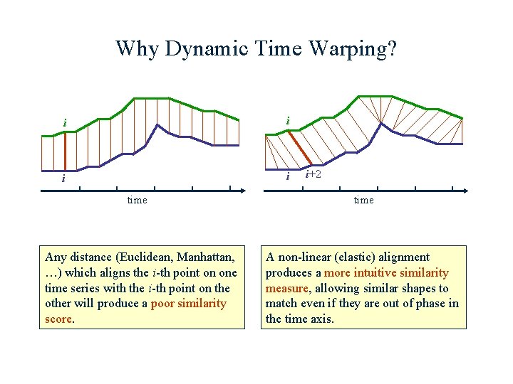
Why Dynamic Time Warping? i i time Any distance (Euclidean, Manhattan, …) which aligns the i-th point on one time series with the i-th point on the other will produce a poor similarity score. i+2 time A non-linear (elastic) alignment produces a more intuitive similarity measure, allowing similar shapes to match even if they are out of phase in the time axis.

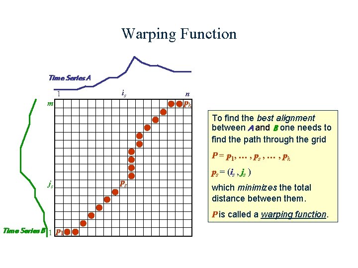
Warping Function Time Series A 1 is m n pk To find the best alignment between A and B one needs to find the path through the grid P = p 1, … , ps , … , pk js ps ps = (is , js ) which minimizes the total distance between them. P is called a warping function. Time Series B 1 p 1

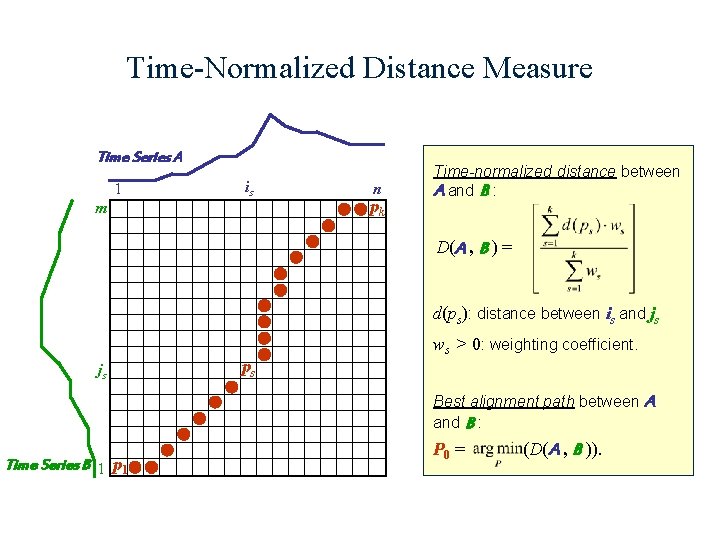
Time-Normalized Distance Measure Time Series A 1 is m n pk Time-normalized distance between A and B : D(A , B ) = d(ps): distance between is and js js ps ws > 0: weighting coefficient. Best alignment path between A and B : Time Series B 1 p 1 P 0 = (D(A , B )).

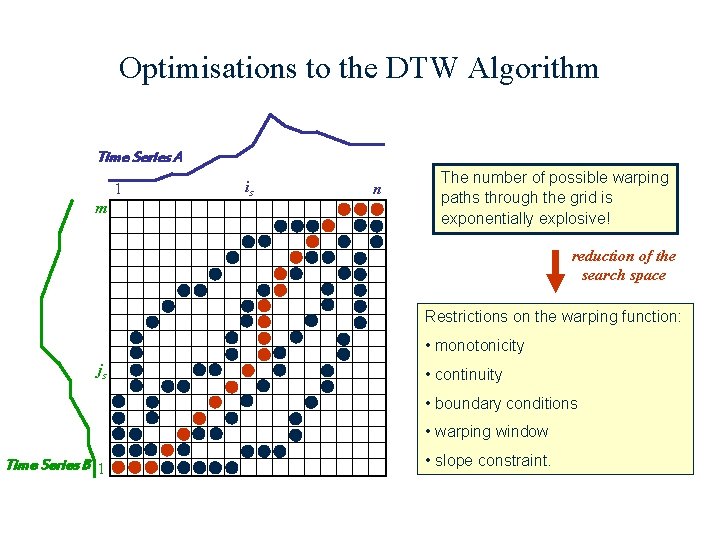
Optimisations to the DTW Algorithm Time Series A 1 m is n The number of possible warping paths through the grid is exponentially explosive! reduction of the search space Restrictions on the warping function: • monotonicity js • continuity • boundary conditions • warping window Time Series B 1 • slope constraint.

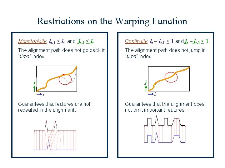
Restrictions on the Warping Function Monotonicity: is-1 ≤ is and js-1 ≤ js. Continuity: is – is-1 ≤ 1 and js – js-1 ≤ 1. The alignment path does not go back in “time” index. The alignment path does not jump in “time” index. j j i Guarantees that features are not repeated in the alignment. i Guarantees that the alignment does not omit important features.

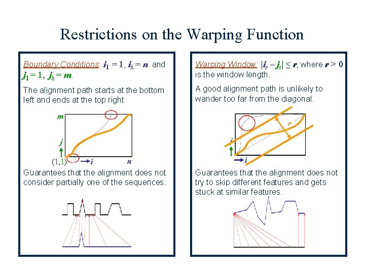
Restrictions on the Warping Function Boundary Conditions: i 1 = 1, ik = n and j 1 = 1, jk = m. Warping Window: |is – js| ≤ r, where r > 0 is the window length. The alignment path starts at the bottom left and ends at the top right. A good alignment path is unlikely to wander too far from the diagonal. m j n (1, 1) i Guarantees that the alignment does not consider partially one of the sequences. r j i Guarantees that the alignment does not try to skip different features and gets stuck at similar features.

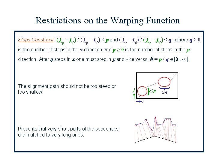
Restrictions on the Warping Function Slope Constraint: ( js – js ) / ( is – is ) ≤ p and ( is – is ) / ( js – js ) ≤ q , where q ≥ 0 p 0 q 0 is the number of steps in the x-direction and p ≥ 0 is the number of steps in the ydirection. After q steps in x one must step in y and vice versa: S = p / q [0 , ]. The alignment path should not be too steep or too shallow. j ≤p i Prevents that very short parts of the sequences are matched to very long ones. ≤q

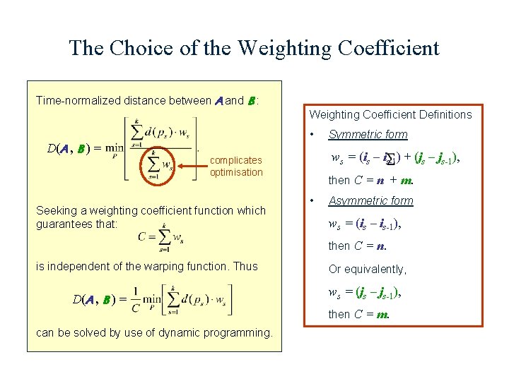
The Choice of the Weighting Coefficient Time-normalized distance between A and B : Weighting Coefficient Definitions • D(A , B ) = ws = (is – is-1) + (js – js-1), complicates optimisation Seeking a weighting coefficient function which guarantees that: Symmetric form then C = n + m. • Asymmetric form ws = (is – is-1), then C = n. is independent of the warping function. Thus D(A , B ) = can be solved by use of dynamic programming. Or equivalently, ws = (js – js-1), then C = m.

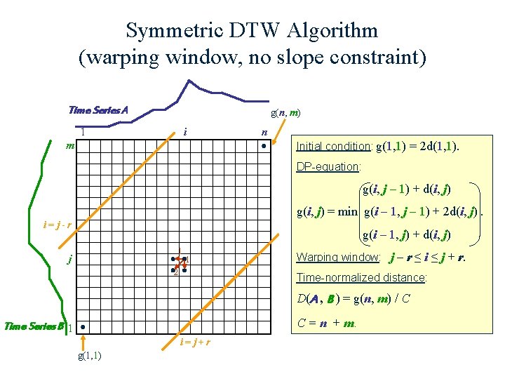
Symmetric DTW Algorithm (warping window, no slope constraint) Time Series A g(n, m) 1 i n Initial condition: g(1, 1) = 2 d(1, 1). m DP-equation: g(i, j – 1) + d(i, j) g(i, j) = min g(i – 1, j – 1) + 2 d(i, j). i=j-r g(i – 1, j) + d(i, j) 2 1 1 j Warping window: j – r ≤ i ≤ j + r. Time-normalized distance: D(A , B ) = g(n, m) / C C = n + m. Time Series B 1 i=j+r g(1, 1)

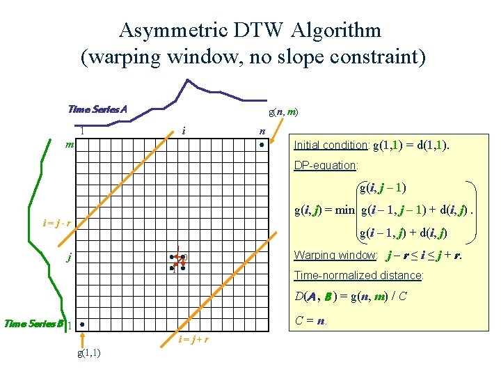
Asymmetric DTW Algorithm (warping window, no slope constraint) Time Series A g(n, m) 1 i n Initial condition: g(1, 1) = d(1, 1). m DP-equation: g(i, j – 1) g(i, j) = min g(i – 1, j – 1) + d(i, j). i=j-r g(i – 1, j) + d(i, j) 1 1 0 j Warping window: j – r ≤ i ≤ j + r. Time-normalized distance: D(A , B ) = g(n, m) / C C = n. Time Series B 1 i=j+r g(1, 1)

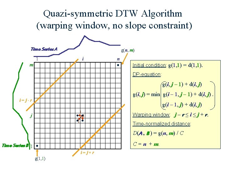
Quazi-symmetric DTW Algorithm (warping window, no slope constraint) Time Series A g(n, m) 1 i n Initial condition: g(1, 1) = d(1, 1). m DP-equation: g(i, j – 1) + d(i, j) g(i, j) = min g(i – 1, j – 1) + d(i, j). i=j-r g(i – 1, j) + d(i, j) 1 1 1 j Warping window: j – r ≤ i ≤ j + r. Time-normalized distance: D(A , B ) = g(n, m) / C C = n + m. Time Series B 1 i=j+r g(1, 1)

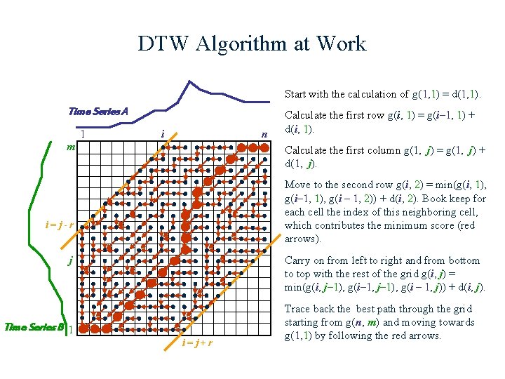
DTW Algorithm at Work Start with the calculation of g(1, 1) = d(1, 1). Time Series A i i=j+r Time Series B 1 j i=j-r m n 1 Calculate the first row g(i, 1) = g(i– 1, 1) + d(i, 1). Calculate the first column g(1, j) = g(1, j) + d(1, j). Move to the second row g(i, 2) = min(g(i, 1), g(i– 1, 1), g(i – 1, 2)) + d(i, 2). Book keep for each cell the index of this neighboring cell, which contributes the minimum score (red arrows). Carry on from left to right and from bottom to top with the rest of the grid g(i, j) = min(g(i, j– 1), g(i– 1, j– 1), g(i – 1, j)) + d(i, j). Trace back the best path through the grid starting from g(n, m) and moving towards g(1, 1) by following the red arrows.

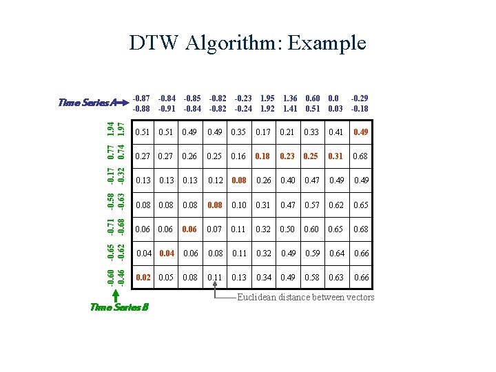
-0. 87 -0. 88 -0. 84 -0. 91 -0. 85 -0. 84 -0. 82 1. 94 1. 97 0. 51 0. 49 0. 35 0. 17 0. 74 0. 27 0. 26 0. 25 0. 16 -0. 17 -0. 32 0. 13 0. 12 -0. 58 -0. 63 0. 08 -0. 71 -0. 68 DTW Algorithm: Example 0. 06 0. 04 0. 02 -0. 60 -0. 65 -0. 46 -0. 62 Time Series A Time Series B -0. 23 -0. 24 1. 95 1. 92 1. 36 1. 41 0. 60 0. 51 0. 03 -0. 29 -0. 18 0. 21 0. 33 0. 41 0. 49 0. 18 0. 23 0. 25 0. 31 0. 68 0. 08 0. 26 0. 40 0. 47 0. 49 0. 08 0. 10 0. 31 0. 47 0. 57 0. 62 0. 65 0. 06 0. 07 0. 11 0. 32 0. 50 0. 65 0. 68 0. 04 0. 06 0. 08 0. 11 0. 32 0. 49 0. 59 0. 64 0. 66 0. 05 0. 08 0. 11 0. 13 0. 34 0. 49 0. 58 0. 63 0. 66 Euclidean distance between vectors