Dynamic Routing Protocols part 3 B Lecture 6

+ Dynamic Routing Protocols part 3 B

+ Lecture 6 Outline Dynamic Routing Protocols Distance Vector Dynamic Routing OSPF RIP Link-State Dynamic Routing

+ OSPF Routing Protocol Components of OSPF Terminologies OSPF Operational State Route calculation and Dijkstra’s Algorithm

+ OSPF Operational States • When an OSPF router is initially connected to a network, it attempts to: ▪ Create adjacencies with neighbors • ▪ Exchange routing information ▪ Calculate the best routes ▪ Reach convergence OSPF router progresses through several states while attempting to reach convergence.

+ Establish Neighbor Adjacencies ■ OSPF-enabled routers must form adjacencies with their neighbor before they can share information with that neighbor. ■ When OSPF is enabled on an interface, the router must determine if there is another OSPF neighbor on the link. ■ To accomplish this, the router forwards a Hello packet that contains its router ID out all OSPF-enabled interfaces to determine whether neighbors are present on those links. ■ If a neighbor is present, the OSPF-enabled router attempts to establish a neighbor adjacency with that neighbor.

+ Establishing Neighbor Adjacencies ■ An OSPF adjacency is established in several steps and OSPF router goes through the following states:

+ Down State ■ This is the first OSPF neighbor adjacency state. ■ It means that no information (Hellos) has been received, but Hello packets can still be sent to the neighbor in this state.

+ Down to Init State ■ In the first step, routers that intend to establish an OSPF neighbor adjacency exchange a Hello packets. * A Cisco router includes the Router IDs of all neighbors in the init (or higher) state in its Hello packets.

+ Init State ■ When a router receives a Hello packet with a router ID that is not within its neighbor list, the receiving router attempts to establish an adjacency with the initiating router. 1 - adds the R 1 router ID to its neighbor list 2 - sends a Hello packet to R 1

+ A router transit to Init State when It is in Down state and it starts sending Hello packet It receives a Hello packet with a router ID that is not within its neighbor list

+ Init State Init state specifies that the router has received a Hello packet from its neighbor, but the receiving router's ID was not included in the hello packet.

+ 2 -Way State ■ When the router sees its own router ID in the Hello packet received from the neighbor, it will transit to the 2 -Way state. ■ This means that bidirectional communication with the neighbor has been established. 1 - adds the R 2 Router ID in its list of OSPF neighbors. 2 - its own Router ID in the Hello packet

+ When a router receives a Hello packet with its Router ID listed in the list of neighbors, it will transit from the Init state to the Two. Way state its Router ID not listed in the list of neighbors, it will transit to the Init state *The transtion to 2 -Way state happens if the router is in the Init state

+ ■ 2 -Way State The action performed in Two-Way state depends on the type of inter-connection between the adjacent routers: ■ If the link is a point-to-point link, then they immediately transition from the Two-Way state to the database synchronization phase. ■ If the routers are interconnected over a multiaccess network, then a designated router(DR) and a backup designated router (BDR) must be elected.

+ ■ Why a DR and a BDR Multiaccess networks can create two challenges : ■ ■ Creation of multiple adjacencies Extensive flooding of LSAs

+ Why a DR and a BDR ■ The solution to managing the number of adjacencies and the flooding of LSAs on a multiaccess network is the DR. ■ On multiaccess networks, OSPF elects a DR to be the collection and distribution point for LSAs sent and received. ■ ■ A BDR is also elected in case the DR fails. All other routers become DROTHERs. A DROTHER is a router that is neither the DR nor the BDR.

+ DR and BDR ■ The DR and BDR act as a central point of contact for link-state information exchange on a multiaccess network. ■ Each router must establish a full adjacency with the DR and the BDR only. ■ Each router, rather than exchanging LSA with every other router on the segment, sends the LSA to the DR and BDR only.

+ DR and BDR DR router performs the following tasks: ■ Network Links Advertisement ■ ■ The DR originates the network LSA for the network. Managing LSDB synchronization: ■ The DR and BDR ensure that the other routers on the network have the same link-state information about the common segment.

+ DR and BDR ■ When the DR is operating, the BDR does not perform any DR functions. ■ Instead, the BDR receives all the information, but the DR performs the LSA forwarding and LSDB synchronization tasks. ■ ■ The BDR performs the DR tasks only if the DR fails. When the DR fails, the BDR automatically becomes the new DR, and a new BDR election occurs.

+ Synchronizing OSPF Databases • After the Two-Way state, routers transition to database synchronization states.

+ Synchronizing OSPF Databases ■ While the Hello packet was used to establish neighbor adjacencies, the other four types of OSPF packets are used during the process of exchanging and synchronizing LSDBs.

+ Ex. Start state ■ In the Ex. Start state, a master and slave relationship is created between each router and its adjacent DR and BDR. ■ The router with the higher router ID acts as the master for the Exchange state.

+ Exchange state ■ In the Exchange state, the master and slave routers exchange one or more DBD packets. ■ DBD packets is an abbreviated list of the sending router’s LSDB and is used by receiving routers to check against the local LSDB. ■ The LSDB must be identical on all OSPF routers within an area to construct an accurate SPF tree.

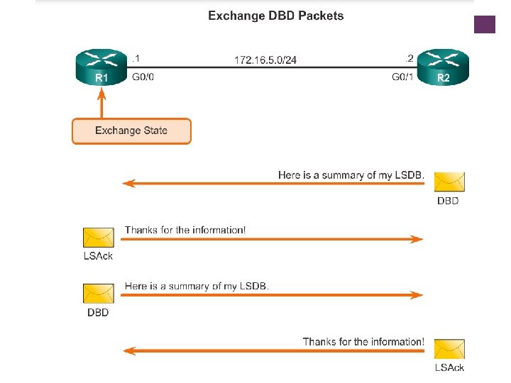
+ Exchange state ■ A DBD packet includes information about the LSA entry header that appears in the router’s LSDB. ■ The entries can be about a link or about a network. ■ Each LSA entry header includes information about the linkstate type, the address of the advertising router, the link’s cost, and the sequence number. ■ The router uses the sequence number to determine the newness of the received link-state information.

+ Loading State ■ When a router receives a DBD packet, it compares the information received with the information it has in its own LSDB. ■ If the DBD packet has a more current LSA or has an LSA that is not in its LSDB, the router transitions to the Loading state.

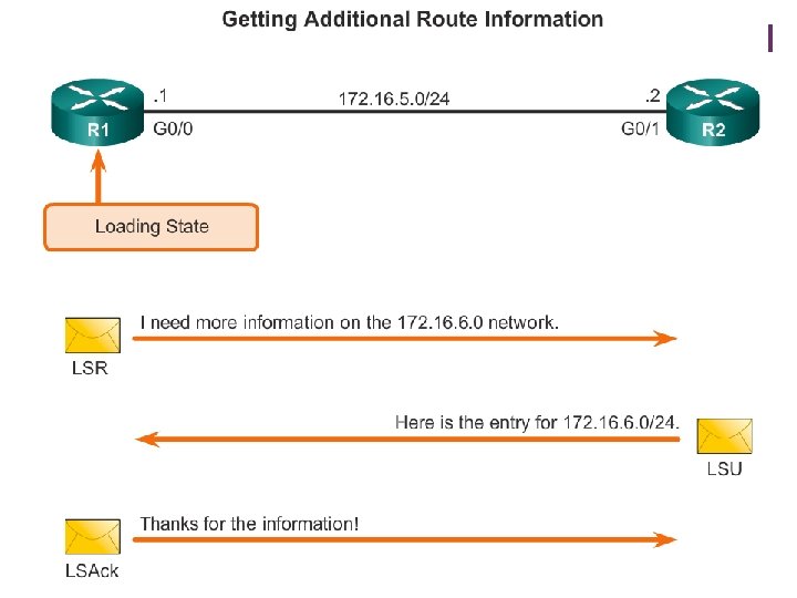
+ Loading State ■ In this state, the actual exchange of link state information occurs. ■ Based on the information provided by the DBDs, routers send link-state request (LSR) packets. ■ The neighbor then provides the requested link-state information in link-state update (LSU) packets. ■ During the adjacency, if a router receives an outdated or missing LSA, it requests that LSA by sending a LSR packet. ■ All link-state update packets are acknowledged.

+ Full State ■ After all LSRs have been satisfied for a given router, the adjacent routers are considered synchronized (have identical LSDBs ) and in a full state.

Establishing Bidirectional Communication Port 2 172. 16. 5. 1/24 A Port 1 172. 16. 5. 2/24 B Down state hello I am router id 172. 16. 5. 1, and I see no one To 224. 0. 0. 5 Initial State Router B neighbor List 172. 16. 5. 1/24, in Port 2 Unicast to A I am router id 172. 16. 5. 2, and I see 172. 16. 5. 1 Router A neighbor List 172. 16. 5. 2/24, in Port 1 Two-way State hello

Discovering the Network Routes Port 2 172. 16. 5. 1/24 A Port 1 172. 16. 5. 2/24 B Exstart state DBD I will start exchange because I have router id 172. 16. 5. 1 No, I’ll start exchange because I have a higher RID DBD exchange State Here is a summary of my LSDB DBD

Adding the Link-State Entries Port 2 172. 16. 5. 1/24 A LSAck Port 1 172. 16. 5. 2/24 Thanks for the information! B LSAck Loading state LSR I need complete entry for network 172. 16. 6. 0/24 Here is the entry for network 172. 16. 6. 0/24 LSAck Thanks for the information! Full State LSU

+ OSPF Routing Protocol Components of OSPF Terminologies OSPF Operational State Route calculation and Dijkstra’s Algorithm

+ From CH 2 p 3 A Slides Previous slides Next slides

+ Route Calculation ■ The router now has a complete LSDB. ■ Now the router is ready to create a routing table, but first needs to run the Shortest Path First (SPF) Algorithm, also called the Dijkstra algorithm, on the LSDB which will create the SPF tree. ■ In the SPF, the router calculations places itself as the root and creating a “tree diagram” of the network

+ Simplified Example ■ In order to keep it simple, we will take some liberties with the actual process and algorithm, but you will get the basic idea! ■ Assume there are 5 Routers that have already established adjacency relationship: ■ Router. A, Router. B, Router. C, Router. D, Router. E

+ Exchanging LSAs and Building LSDB ■ ■ Router. A LSA , which will be flooded to all other routers: ■ Router. B on your network 11. 0. 0. 0/8 with a cost of 15, ■ Router. C on your network 12. 0. 0. 0/8 with a cost of 2 ■ Router. D on your network 13. 0. 0. 0/8 with a cost of 5 ■ Have a “leaf” network 10. 0/8 with a cost of 2 All other routers will also flood their link state information. (OSPF: only within the area) 11. 0. 0. 0/8 “Leaf” 10. 0/8 12. 0. 0. 0/8 2 13. 0. 0. 0/8

+ Exchanging LSAs and Building LSDB Router. B: Router. A’s LSDB ■ Connected to Router. A on network 11. 0. 0. 0/8, cost of 15 ■ Connected to Router. E on network 15. 0. 0. 0/8, cost of 2 ■ Has a “leaf” network 14. 0. 0. 0/8, cost of 15 Router. C: • All other routers flood their own LSA to all other routers. • Router. A gets all of this information and stores it in its LSDB. • Using the LSA from each router, Router. A runs Dijkstra algorithm to create a SPT. ■ Connected to Router. A on network 12. 0. 0. 0/8, cost of 2 ■ Connected to Router. D on network 16. 0. 0. 0/8, cost of 2 ■ Has a “leaf” network 17. 0. 0. 0/8, cost of 2 Router. D: ■ Connected to Router. A on network 13. 0. 0. 0/8, cost of 5 ■ Connected to Router. C on network 16. 0. 0. 0/8, cost of 2 ■ Connected to Router. E on network 18. 0. 0. 0/8, cost of 2 ■ Has a “leaf” network 19. 0. 0. 0/8, cost of 2 Router. E: ■ Connected to Router. B on network 15. 0. 0. 0/8, cost of 2 ■ Connected to Router. D on network 18. 0. 0. 0/8, cost of 10 ■ Has a “leaf” network 20. 0/8, cost of 2

+ Link State information from Router. B LSA : 14. 0. 0. 0/8 ■ Connected to Router. A on network 11. 0. 0. 0/8, cost of 15 ■ Connected to Router. E on network 15. 0. 0. 0/8, cost of 2 ■ Have a “leaf” network 14. 0. 0. 0/8, cost of 2 2 11. 0. 0. 0/8 Now, Router. A attaches the two graphs… 15. 0. 0. 0/8 14. 0. 0. 0/8 2 14. 0. 0. 0/8 11. 0. 0. 0/8 10. 0/8 12. 0. 0. 0/8 2 + 2 15. 0. 0. 0/8 11. 0. 0. 0/8 = 10. 0/8 12. 0. 0. 0/8 2 13. 0. 0. 0/8 15. 0. 0. 0/8

+ Link State information from Router. C LSA : ■ 12. 0. 0. 0/8 Connected to Router. A on network 12. 0. 0. 0/8, cost of 2 ■ Connected to Router. D on network 16. 0. 0. 0/8, cost of 2 ■ Have a “leaf” network 17. 0. 0. 0/8, cost of 2 14. 0. 0. 0/8 2 11. 0. 0. 0/8 2 16. 0. 0. 0/8 Now, Router. A attaches the two graphs… 15. 0. 0. 0/8 17. 0. 0. 0/8 10. 0/8 12. 0. 0. 0/8 2 13. 0. 0. 0/8 17. 0. 0. 0/8 + 14. 0. 0. 0/8 2 2 16. 0. 0. 0/8 11. 0. 0. 0/8 10. 0/8 = 15. 0. 0. 0/8 12. 0. 0. 0/8 2 17. 0. 0. 0/8 16. 0. 0. 0/8 13. 0. 0. 0/8

+ Link State information from Router. D From Router. D LSA : ■ Connected to Router. A on network 13. 0. 0. 0/8, cost of 5 ■ Connected to Router. C on network 16. 0. 0. 0/8, cost of 2 ■ Connected to Router. E on network 18. 0. 0. 0/8, cost of 10 ■ Have a “leaf” network 19. 0. 0. 0/8, cost of 2 16. 0. 0. 0/8 13. 0. 0. 0/8 18. 0. 0. 0/8 2 19. 0. 0. 0/8 Now, Router. A attaches the two graphs… 14. 0. 0. 0/8 2 11. 0. 0. 0/8 15. 0. 0. 0/8 11. 0. 0. 0/8 18. 0. 0. 0/8 10. 0/8 12. 0. 0. 0/8 2 17. 0. 0. 0/8 16. 0. 0. 0/8 + 2 19. 0. 0. 0/8 15. 0. 0. 0/8 12. 0. 0. 0/8 10. 0/8 = 2 17. 0. 0. 0/8 16. 0. 0. 0/8 13. 0. 0. 0/8 18. 0. 0. 0/8 2 19. 0. 0. 0/8

+ Link State information from Router. E From Router. E LSA : 15. 0. 0. 0/8 ■ Connected to Router. B on network 15. 0. 0. 0/8, cost of 2 ■ Connected to Router. D on network 18. 0. 0. 0/8, cost of 10 ■ Have a “leaf” network 20. 0/8, cost of 2 20. 0/8 2 18. 0. 0. 0/8 14. 0. 0. 0/8 2 11. 0. 0. 0/8 Now, Router. A attaches the two graphs… 14. 0. 0. 0/8 15. 0. 0. 0/8 2 12. 0. 0. 0/8 10. 0/8 2 17. 0. 0. 0/8 16. 0. 0. 0/8 + 11. 0. 0. 0/8 20. 0/8 2 10. 0/8 13. 0. 0. 0/8 18. 0. 0. 0/8 2 15. 0. 0. 0/8 12. 0. 0. 0/8 2 20. 0/8 17. 0. 0. 0/8 2 16. 0. 0. 0/8 19. 0. 0. 0/8 13. 0. 0. 0/8 18. 0. 0. 0/8 2 19. 0. 0. 0/8

+ Topology ■ Using the LSDB content, Router. A has now built a complete topology of the network. ■ The next step for OSPF is to find the best path to each node and leaf network. 14. 0. 0. 0/8 2 11. 0. 0. 0/8 15. 0. 0. 0/8 12. 0. 0. 0/8 10. 0/8 20. 0/8 17. 0. 0. 0/8 2 2 2 16. 0. 0. 0/8 13. 0. 0. 0/8 18. 0. 0. 0/8 2 19. 0. 0. 0/8

+ Choosing the Best Path ■ Using the Dijkstra’s algorithm Router. A can now proceed to find the shortest path to each leaf network

+ SPT Results Put into the Routing Table Router. A’s Routing Table 10. 0/8 11. 0. 0. 0/8 connected e 0 connected s 0 12. 0. 0. 0/8 13. 0. 0. 0/8 connected s 1 connected s 2 14. 0. 0. 0/8 2 11. 0. 0. 0/8 14. 0. 0. 0/8 17 s 0 15. 0. 0. 0/8 16 s 1 16. 0. 0. 0/8 4 s 1 17. 0. 0. 0/8 4 s 1 10. 0/8 18. 0. 0. 0/8 19. 0. 0. 0/8 20. 0/8 14 s 1 6 s 1 16 s 1 e 0 s 0 15. 0. 0. 0/8 12. 0. 0. 0/8 s 1 20. 0/8 17. 0. 0. 0/8 2 2 16. 0. 0. 0/8 s 2 18. 0. 0. 0/8 13. 0. 0. 0/8 2 19. 0. 0. 0/8

+ If a link fail ■ When change occurs: ■ Announce the change to all OSPF neighbours ■ ■ All routers run the SPF algorithm on the revised database Install any change in the routing table

+ Dijkstra Algorithm Notation

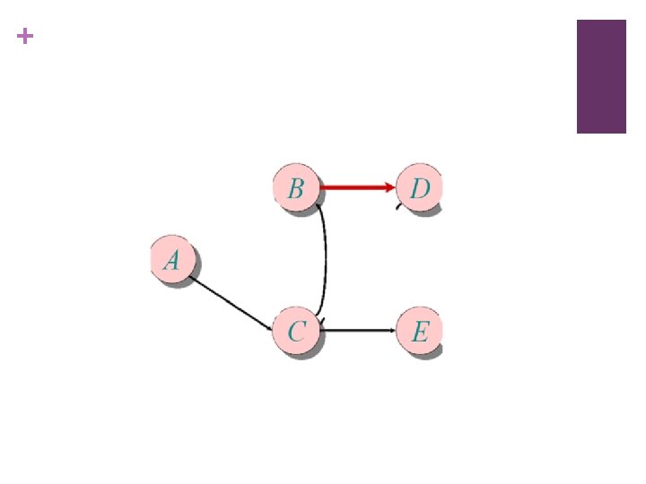
+ ijkstra Animated Example D

+ ijkstra Animated Example D

+ ijkstra Animated Example D

+ ijkstra Animated Example D C C C

+ ijkstra Animated Example D C C C

+ ijkstra Animated Example D C C C

+ ijkstra Animated Example D C C C

+ ijkstra Animated Example D C C B C

+ ijkstra Animated Example D C C B C