Dynamic Response Unit step signal Step response ysHss

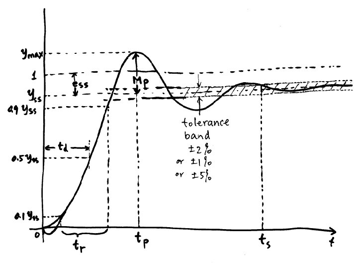
Dynamic Response • Unit step signal: • Step response: y(s)=H(s)/s, y(t)=L-1{H(s)/s} Time domain response specifications • Defined based on unit step response • Defined for closed-loop system

By final value theorem In MATLAB: num = [. . . . ]; den=[……]; b 0 = num(end); a 0 = den(end); yss=b 0/a 0;

If numerical values of y and t available, from [y, t]=step(num, den); abs(y – yss) < tol means inside band abs(y – yss) ≥ tol not inside e. g. t_out = t(abs(y – yss) >= tol) contains all those time points when y is not inside the band. Therefore, the last value in t_out will be the settling time. ts=t_out(end)

Peak time tp = time when y(t) reaches its maximum value. Peak value ymax = y(tp) Hence: ymax = max(y); tp = t(y == ymax); Overshoot: OS = ymax - yss Percentage overshoot:

If t 50 = t(y >= 0. 5*yss), this contains all time points when y(t) is ≥ 50% of yss so the first such point is td. td=t 50(1); Similarly, t 10 = t(y >= 0. 1*yss) & t 90 = t(y >= 0. 9*yss) can be used to find tr. tr=t 90(1)-t 10(1)

tp=0. 35 ts≈0. 92 O. S. =0. 4 Mp=40% yss=1 ess=0 td≈0. 2 tr≈0. 1

Transient Response • First order system transient response – Step response specs and relationship to pole location • Second order system transient response – Step response specs and relationship to pole location • Effects of additional poles and zeros

Prototype first order system E U(s) + - 1 τs Y(s)

First order system step resp Normalized time t/t

Prototype first order system • • • No overshoot, tp=inf, Mp = 0 Yss=1, ess=0 Settling time ts = [-ln(tol)]/p Delay time td = [-ln(0. 5)]/p Rise time tr = [ln(0. 9) – ln(0. 1)]/p • All times proportional to 1/p= t • Larger p means faster response

The error signal: e(t) = 1 -y(t)=e-ptus(t) Normalized time t/t

In every τ seconds, the error is reduced by 63. 2%

General First-order system We know how this responds to input Step response starts at y(0+)=k, final value kz/p 1/p = t is still time constant; in every t, y(t) moves 63. 2% closer to final value

Step response by MATLAB: >> p =. . >> n = [ b 1 b 0 ] >> d = [ 1 p ] >> step ( n , d ) Other MATLAB commands to explore: plot, hold, axis, xlabel, ylabel, title, text, gtext, semilogx, semilogy, loglog, subplot

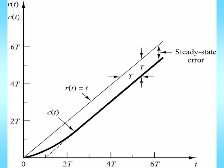
Unit ramp response:

Note: In step response, the steady-state tracking error = zero.

Unit impulse response:

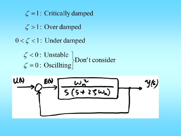
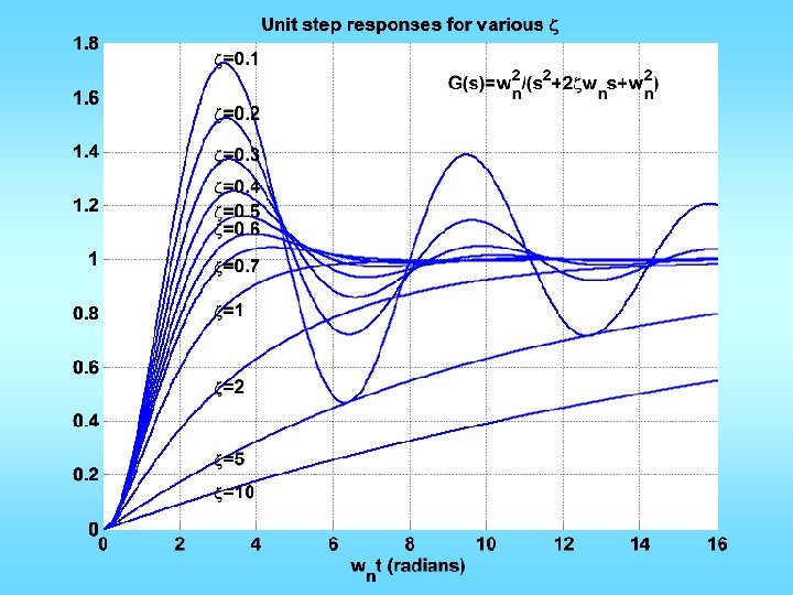
Prototype nd 2 order system:

xi=[0. 7 1 2 5 10 0. 1 0. 2 0. 3 0. 4 0. 5 0. 6]; x=['zeta=0. 7'; 'zeta=1 '; 'zeta=2 '; 'zeta=5 '; 'zeta=10 '; 'zeta=0. 1'; 'zeta=0. 2'; 'zeta=0. 3'; 'zeta=0. 4'; 'zeta=0. 5'; 'zeta=0. 6']; T=0: 0. 01: 16; figure; hold; for k=1: length(xi) n=[1]; d=[1 2*xi(k) 1]; y=step(n, d, T); plot(T, y); if xi(k)>=0. 7 text(T(290), y(310), x(k, : )); else text(T(290), max(y)+0. 02, x(k, : )); end grid; end text(9, 1. 65, 'G(s)=w_n^2/(s^2+2zetaw_ns+w_n^2)') title('Unit step responses for various zeta') xlabel('w_nt (radians)') Can use omega in stead of w

annotation Create annotations including lines, arrows, text arrows, double arrows, text boxes, rectangles, and ellipses xlabel, ylabel, zlabel Add a text label to the respective axis title Add a title to a graph colorbar Add a colorbar to a graph legend Add a legend to a graph

For example: “help annotation” explains how to use the annotation command to add text, lines, arrows, and so on at desired positions in the graph ANNOTATION('textbox', POSITION) creates a textbox annotation at the position specified in normalized figure units by the vector POSITION ANNOTATION('line', X, Y) creates a line annotation with endpoints specified in normalized figure coordinates by the vectors X and Y ANNOTATION('arrow', X, Y) creates an arrow annotation with endpoints specified Example: ah=annotation('arrow', [. 9. 5], [. 9, . 5], 'Color', 'r'); th=annotation('textarrow', [. 3, . 6], [. 7, . 4], 'String', 'ABC');