Dynamic Programming Several problems Principle of dynamic programming

Dynamic Programming • Several problems • Principle of dynamic programming - Optimal substructure - Recursive solution - Computation of optimal solution • Longest Common Subsequences • Optimal binary search trees Jan. 2018

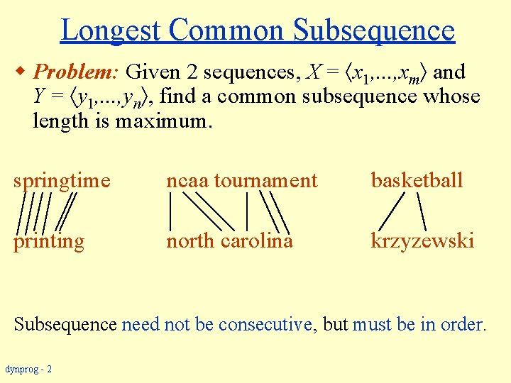
Longest Common Subsequence w Problem: Given 2 sequences, X = x 1, . . . , xm and Y = y 1, . . . , yn , find a common subsequence whose length is maximum. springtime ncaa tournament basketball printing north carolina krzyzewski Subsequence need not be consecutive, but must be in order. dynprog - 2

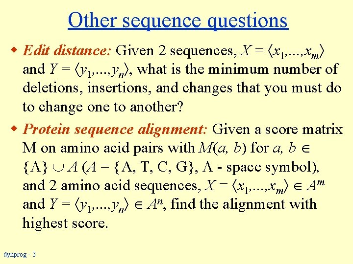
Other sequence questions w Edit distance: Given 2 sequences, X = x 1, . . . , xm and Y = y 1, . . . , yn , what is the minimum number of deletions, insertions, and changes that you must do to change one to another? w Protein sequence alignment: Given a score matrix M on amino acid pairs with M(a, b) for a, b { } A (A = {A, T, C, G}, - space symbol), and 2 amino acid sequences, X = x 1, . . . , xm Am and Y = y 1, . . . , yn An, find the alignment with highest score. dynprog - 3

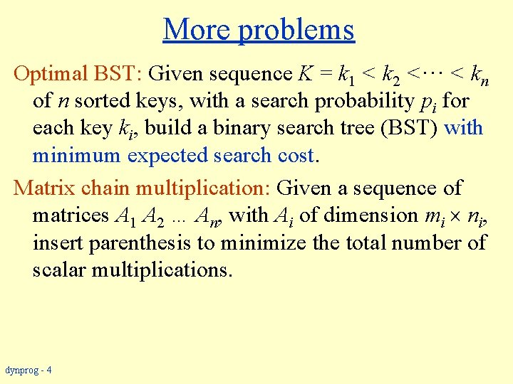
More problems Optimal BST: Given sequence K = k 1 < k 2 <··· < kn of n sorted keys, with a search probability pi for each key ki, build a binary search tree (BST) with minimum expected search cost. Matrix chain multiplication: Given a sequence of matrices A 1 A 2 … An, with Ai of dimension mi ni, insert parenthesis to minimize the total number of scalar multiplications. dynprog - 4

Dynamic Programming w Dynamic Programming is an algorithm design technique for optimization problems: often minimizing or maximizing. w Like divide and conquer, DP solves problems by combining solutions to subproblems. w Unlike divide and conquer, subproblems are not independent. » Subproblems may share subsubproblems, » However, solution to one subproblem may not affect the solutions to other subproblems of the same problem. (More on this later. ) w DP reduces computation by » Solving subproblems in a bottom-up fashion. » Storing solution to a subproblem the first time it is solved. » Looking up the solution when subproblem is encountered again. w Key: determine structure of optimal solutions dynprog - 5

Steps in Dynamic Programming 1. Characterize structure of an optimal solution. 2. Define value of optimal solution recursively. 3. Compute optimal solution values either topdown with caching or bottom-up in a table. 4. Construct an optimal solution from computed values. We’ll study these with the help of examples. dynprog - 6

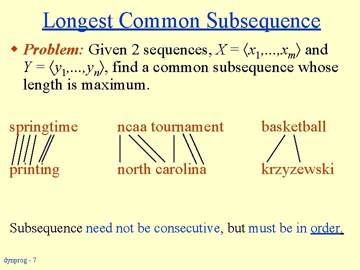
Longest Common Subsequence w Problem: Given 2 sequences, X = x 1, . . . , xm and Y = y 1, . . . , yn , find a common subsequence whose length is maximum. springtime ncaa tournament basketball printing north carolina krzyzewski Subsequence need not be consecutive, but must be in order. dynprog - 7

Naïve Algorithm w For every subsequence of X, check whether it’s a subsequence of Y. w Time: Θ(n 2 m). » 2 m subsequences of X to check. » Each subsequence takes Θ(n) time to check: scan Y for first letter, for second, and so on. dynprog - 8

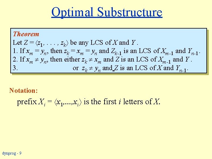
Optimal Substructure Theorem Let Z = z 1, . . . , zk be any LCS of X and Y. 1. If xm = yn, then zk = xm = yn and Zk-1 is an LCS of Xm-1 and Yn-1. 2. If xm yn, then either zk xm and Z is an LCS of Xm-1 and Y. 3. or zk yn and Z is an LCS of X and Yn-1. Notation: prefix Xi = x 1, . . . , xi is the first i letters of X. dynprog - 9

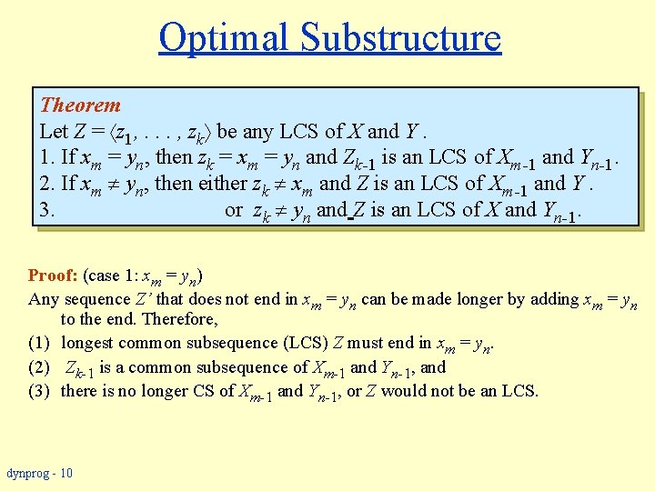
Optimal Substructure Theorem Let Z = z 1, . . . , zk be any LCS of X and Y. 1. If xm = yn, then zk = xm = yn and Zk-1 is an LCS of Xm-1 and Yn-1. 2. If xm yn, then either zk xm and Z is an LCS of Xm-1 and Y. 3. or zk yn and Z is an LCS of X and Yn-1. Proof: (case 1: xm = yn) Any sequence Z’ that does not end in xm = yn can be made longer by adding xm = yn to the end. Therefore, (1) longest common subsequence (LCS) Z must end in xm = yn. (2) Zk-1 is a common subsequence of Xm-1 and Yn-1, and (3) there is no longer CS of Xm-1 and Yn-1, or Z would not be an LCS. dynprog - 10

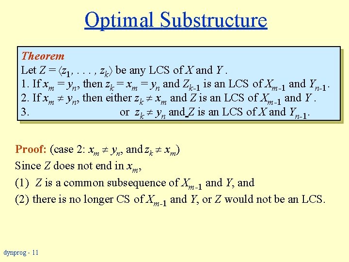
Optimal Substructure Theorem Let Z = z 1, . . . , zk be any LCS of X and Y. 1. If xm = yn, then zk = xm = yn and Zk-1 is an LCS of Xm-1 and Yn-1. 2. If xm yn, then either zk xm and Z is an LCS of Xm-1 and Y. 3. or zk yn and Z is an LCS of X and Yn-1. Proof: (case 2: xm yn, and zk xm) Since Z does not end in xm, (1) Z is a common subsequence of Xm-1 and Y, and (2) there is no longer CS of Xm-1 and Y, or Z would not be an LCS. dynprog - 11

Recursive Solution w Define c[i, j] = length of LCS of Xi and Yj. w We want to get c[m, n]. This gives a recursive algorithm and solves the problem. But does it solve it well? dynprog - 12

Recursive Solution c[springtime, printing] same c[springtim, printing] c[springtime, printin] subproblem [springti, printing] [springtim, printin] [springtime, printi] [springt, printing] [springti, printin] [springtim, printi] [springtime, print] dynprog - 13

Recursive Solution • Keep track of c[a, b] in a table of nm entries: 0 s 0 • top/down p 0 • bottom/up r 0 i 0 n 0 g 0 t 0 i 0 m 0 dynprog - 14 e 0 p r i n t i n g 0 0 0 0

Computing the length of an LCS-LENGTH (X, Y) 1. m ← length[X] 2. n ← length[Y] 3. for i ← 1 to m initialization 4. do c[i, 0] ← 0 5. for j ← 0 to n 6. do c[0, j ] ← 0 7. for i ← 1 to m 8. do for j ← 1 to n 9. do if xi = yj 10. then c[i, j ] ← c[i 1, j 1] + 1 11. b[i, j ] ← “ ” 12. else if c[i 1, j ] ≥ c[i, j 1] 13. then c[i, j ] ← c[i 1, j ] 14. b[i, j ] ← “↑” 15. else c[i, j ] ← c[i, j 1] 16. b[i, j ] ← “←” 17. return c and b dynprog - 15 b[i, j] points to table entry whose subproblem we used in solving LCS of Xi and Yj. i – 1, j i, j -1 c[m, n] contains the length of an LCS of X and Y. Time: O(mn)

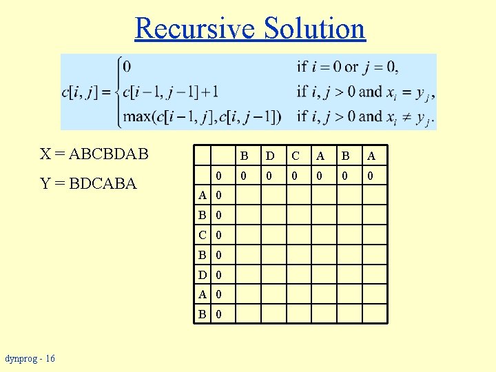
Recursive Solution X = ABCBDAB Y = BDCABA 0 B D C A B A 0 0 0 A 0 B 0 C 0 B 0 D 0 A 0 B 0 dynprog - 16

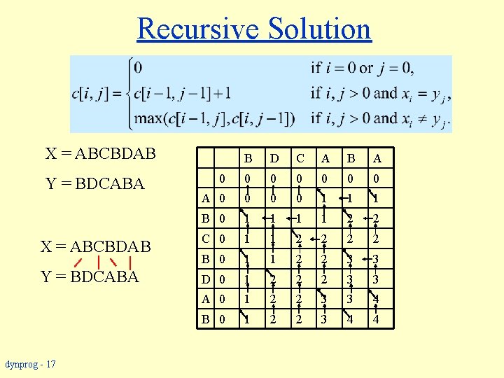
Recursive Solution X = ABCBDAB B D C A B A 0 0 0 0 A 0 0 1 1 1 B 0 1 1 2 2 X = ABCBDAB C 0 1 1 2 2 B 0 1 1 2 2 3 3 Y = BDCABA D 0 1 2 2 2 3 3 A 0 1 2 2 3 3 4 B 0 1 2 2 3 4 4 Y = BDCABA dynprog - 17

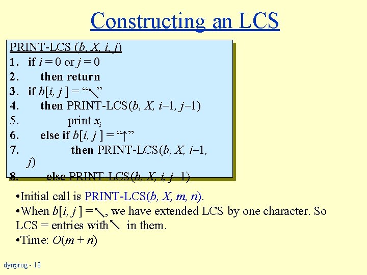
Constructing an LCS PRINT-LCS (b, X, i, j) 1. if i = 0 or j = 0 2. then return 3. if b[i, j ] = “ ” 4. then PRINT-LCS(b, X, i 1, j 1) 5. print xi 6. else if b[i, j ] = “↑” 7. then PRINT-LCS(b, X, i 1, j) 8. else PRINT-LCS(b, X, i, j 1) • Initial call is PRINT-LCS(b, X, m, n). • When b[i, j ] = , we have extended LCS by one character. So LCS = entries with in them. • Time: O(m + n) dynprog - 18

Steps in Dynamic Programming 1. Characterize structure of an optimal solution. 2. Define value of optimal solution recursively. 3. Compute optimal solution values either topdown with caching or bottom-up in a table. 4. Construct an optimal solution from computed values. We’ll study these with the help of examples. dynprog - 19

Optimal Binary Search Trees w Problem » Given sequence K = k 1 < k 2 <··· < kn of n sorted keys, with a search probability pi for each key ki. » Want to build a binary search tree (BST) with minimum expected search cost. » Actual cost = # of items examined. » For key ki, cost(ki) = depth. T(ki) +1, where depth. T(ki) = depth of ki in BST T. dynprog - 20

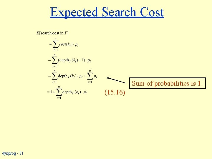
Expected Search Cost Sum of probabilities is 1. (15. 16) dynprog - 21

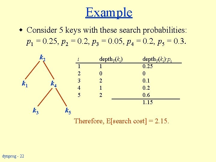
Example w Consider 5 keys with these search probabilities: p 1 = 0. 25, p 2 = 0. 2, p 3 = 0. 05, p 4 = 0. 2, p 5 = 0. 3. k 2 k 1 i depth. T(ki) 1 1 2 0 3 2 4 1 5 2 k 4 k 3 depth. T(ki)·pi 0. 25 0 0. 1 0. 2 0. 6 1. 15 k 5 Therefore, E[search cost] = 2. 15. dynprog - 22

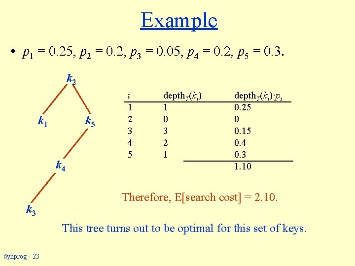
Example w p 1 = 0. 25, p 2 = 0. 2, p 3 = 0. 05, p 4 = 0. 2, p 5 = 0. 3. k 2 k 1 k 5 k 4 k 3 i depth. T(ki) 1 1 2 0 3 3 4 2 5 1 depth. T(ki)·pi 0. 25 0 0. 15 0. 4 0. 3 1. 10 Therefore, E[search cost] = 2. 10. This tree turns out to be optimal for this set of keys. dynprog - 23

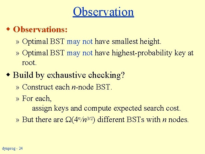
Observation w Observations: » Optimal BST may not have smallest height. » Optimal BST may not have highest-probability key at root. w Build by exhaustive checking? » Construct each n-node BST. » For each, assign keys and compute expected search cost. » But there are (4 n/n 3/2) different BSTs with n nodes. dynprog - 24

Optimal Substructure w Any subtree of a BST contains keys in a contiguous range ki, . . . , kj for some 1 ≤ i ≤ j ≤ n. T T w If T is an optimal BST and T contains subtree T with keys ki, . . . , kj , then T must be an optimal BST for keys ki, . . . , kj. w Proof: … …. dynprog - 25

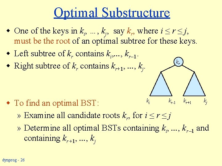
Optimal Substructure w One of the keys in ki, …, kj, say kr, where i ≤ r ≤ j, must be the root of an optimal subtree for these keys. w Left subtree of kr contains ki, . . . , kr 1. kr w Right subtree of kr contains kr+1, . . . , kj. ki kr-1 kr+1 kj w To find an optimal BST: » Examine all candidate roots kr, for i ≤ r ≤ j » Determine all optimal BSTs containing ki, . . . , kr 1 and containing kr+1, . . . , kj dynprog - 26

Recursive Solution w Find optimal BST for ki, . . . , kj, where i ≥ 1, j ≤ n, j ≥ i 1. When j = i 1, the tree is empty. w Define e[i, j] = expected search cost of optimal BST for ki, . . . , kj. w If j = i 1, then e[i, j] = 0. w If j ≥ i, » Select a root kr, for some i ≤ r ≤ j. » Recursively make an optimal BSTs • for ki, . . , kr 1 as the left subtree, e[i, r - 1] and • for kr+1, . . . , kj as the right subtree, e[r + 1, j]. dynprog - 27

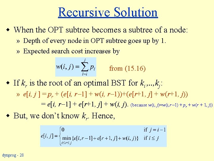
Recursive Solution w When the OPT subtree becomes a subtree of a node: » Depth of every node in OPT subtree goes up by 1. » Expected search cost increases by from (15. 16) w If kr is the root of an optimal BST for ki , . . , kj: » e[i, j ] = pr + (e[i, r 1] + w(i, r 1))+(e[r+1, j] + w(r+1, j)) = e[i, r 1] + e[r+1, j] + w(i, j). (because w(i, j)=w(i, r 1) + pr + w(r + 1, j)) w But, we don’t know kr. Hence, dynprog - 28

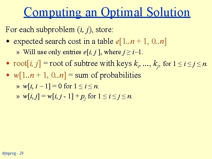
Computing an Optimal Solution For each subproblem (i, j), store: w expected search cost in a table e[1. . n + 1, 0. . n] » Will use only entries e[i, j ], where j ≥ i 1. w root[i, j] = root of subtree with keys ki, . . . , kj, for 1 ≤ i ≤ j ≤ n. w w[1. . n + 1, 0. . n] = sum of probabilities » w[i, i 1] = 0 for 1 ≤ i ≤ n. » w[i, j] = w[i, j - 1] + pj for 1 ≤ i ≤ j ≤ n. dynprog - 29

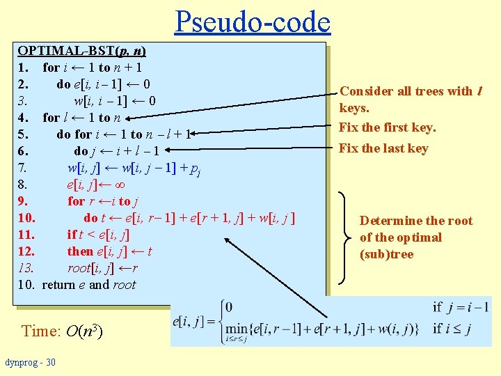
Pseudo-code OPTIMAL-BST(p, n) 1. for i ← 1 to n + 1 2. do e[i, i 1] ← 0 3. w[i, i 1] ← 0 4. for l ← 1 to n 5. do for i ← 1 to n l + 1 6. do j ← i + l 1 7. w[i, j] ← w[i, j 1] + pj 8. e[i, j]← ∞ 9. for r ←i to j 10. do t ← e[i, r 1] + e[r + 1, j] + w[i, j ] 11. if t < e[i, j] 12. then e[i, j] ← t 13. root[i, j] ←r 10. return e and root Time: O(n 3) dynprog - 30 Consider all trees with l keys. Fix the first key. Fix the last key Determine the root of the optimal (sub)tree

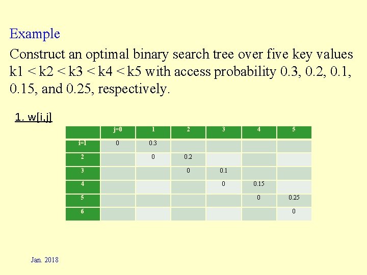
Example Construct an optimal binary search tree over five key values k 1 < k 2 < k 3 < k 4 < k 5 with access probability 0. 3, 0. 2, 0. 1, 0. 15, and 0. 25, respectively. 1. w[i, j] Jan. 2018 j=0 1 2 3 4 5 i=1 0 0. 3 2 0 0. 2 3 0 0. 1 4 0 0. 15 5 0 0. 25 6 0

1. e[i, j] i=1 2 3 4 5 6 j=0 0 1 0. 3 0 2 0. 2 0 3 0. 1 0 i=1 2 3 4 5 6 j=0 1 1 2 2 3 3 4 0. 15 0 5 0. 25 0 1. r[i, j] dynprog - 32 4 4 5

2. w[i, j] i=1 2 3 4 5 6 j=0 0 1 0. 3 0 2 0. 5 0. 2 0 3 0. 3 0. 1 0 4 0. 25 0. 15 0 5 0. 4 0. 25 0 i=1 2 3 4 5 6 j=0 0 1 0. 3 0 2 0. 7 0. 2 0 3 0. 4 0. 1 0 4 0. 35 0. 15 0 5 0. 55 0. 25 0 i=1 2 3 4 5 6 j=0 1 1 2 1 2 3 2 3 4 4 4 5 5 5 2. e[i, j] 2. r[i, j] dynprog - 33

3. w[i, j] i=1 2 3 4 5 6 j=0 0 1 0. 3 0 2 0. 5 0. 2 0 3 0. 6 0. 3 0. 1 0 4 0. 45 0. 25 0. 15 0 5 0. 4 0. 25 0 3. e[i, j] i=1 2 3 4 5 6 j=0 0 1 0. 3 0 2 0. 7 0. 2 0 3 1 0. 4 0. 1 0 4 0. 8 0. 35 0. 15 0 5 0. 85 0. 55 0. 25 0 i=1 2 3 4 5 6 j=0 1 1 2 1 2 3 2 2 3 4 3 4 4 5 5 3. r[i, j] dynprog - 34

4. w[i, j] i=1 2 3 4 5 6 j=0 0 1 0. 3 0 2 0. 5 0. 2 0 3 0. 6 0. 3 0. 1 0 4 0. 75 0. 45 0. 25 0. 15 0 5 0. 7 0. 5 0. 4 0. 25 0 i=1 2 3 4 5 6 j=0 0 1 0. 3 0 2 0. 7 0. 2 0 3 1 0. 4 0. 1 0 4 1. 4 0. 8 0. 35 0. 15 0 5 1. 35 0. 85 0. 55 0. 25 0 i=1 2 3 4 5 6 j=0 1 1 2 1 2 3 2 2 3 4 2 3 4 4 5 5 5 4. e[i, j] 4. r[i, j] dynprog - 35

5. w[i, j] i=1 2 3 4 5 6 j=0 0 1 0. 3 0 2 0. 5 0. 2 0 3 0. 6 0. 3 0. 1 0 4 0. 75 0. 45 0. 25 0. 15 0 5 1 0. 7 0. 5 0. 4 0. 25 0 i=1 2 3 4 5 6 j=0 0 1 0. 3 0 2 0. 7 0. 2 0 3 1 0. 4 0. 1 0 4 1. 4 0. 8 0. 35 0. 15 0 5 2. 15 1. 35 0. 85 0. 55 0. 25 0 i=1 2 3 4 5 6 j=0 1 1 2 1 2 3 1 2 3 4 2 2 4 4 5 5 5. e[i, j] 5. r[i, j] Jan. 2018

r[1, 5] = 2 shows that the root of the tree over k 1, k 2, k 3, k 4, k 5 is k 2 k 1 k 3, k 4, k 5 r[3, 5] = 4 shows that the root of the subtree over k 3, k 4, k 5 is k 4. k 2 k 4 k 1 k 3 k 5 k 3 dynprog - 37 k 5

Elements of Dynamic Programming w Optimal substructure w Overlapping subproblems dynprog - 38

Optimal Substructure w Show that a solution to a problem consists of making a choice, which leaves one or more subproblems to solve. w Suppose that you are given this last choice that leads to an optimal solution. w Given this choice, determine which subproblems arise and how to characterize the resulting space of subproblems. w Show that the solutions to the subproblems used within the optimal solution must themselves be optimal. Usually use cut-and-paste. w Need to ensure that a wide enough range of choices and subproblems are considered. dynprog - 39

Optimal Substructure w Optimal substructure varies across problem domains: » 1. How many subproblems are used in an optimal solution. » 2. How many choices in determining which subproblem(s) to use. w Informally, running time depends on (# of subproblems overall) (# of choices). w How many subproblems and choices do the examples considered contain? w Dynamic programming uses optimal substructure bottom up. » First find optimal solutions to subproblems. » Then choose which to use in optimal solution to the problem. dynprog - 40

Optimal Substucture w Does optimal substructure apply to all optimization problems? No. w Applies to determining the shortest path but NOT the longest simple path of an unweighted directed graph. w Why? » Shortest path has independent subproblems. » Solution to one subproblem does not affect solution to another subproblem of the same problem. » Subproblems are not independent in longest simple path. • Solution to one subproblem affects the solutions to other subproblems. » Example: dynprog - 41

Overlapping Subproblems w The space of subproblems must be “small”. w The total number of distinct subproblems is a polynomial in the input size. » A recursive algorithm is exponential because it solves the same problems repeatedly. » If divide-and-conquer is applicable, then each problem solved will be brand new. dynprog - 42