Dynamic Programming Search for Continuous Speech Recognition 2004113

Dynamic Programming Search for Continuous Speech Recognition 2004/11/3 報告者：陳怡婷

Concerned Problems Could this huge search space be handled by DP in an efficient way? n How to decide good DP search n DP computes only the single best sentence? ? n

Outline Describe some problems and rule about Speech recognition n One-Pass DP Search Using a Linear Lexicon n One-Pass DP Search Using a Tree Lexicon n One-Pass DP Search for Word Graph Construction n

Boundary of Acoustic signal or words、 speakers、quality of speech signal、naturallanguage… n Bayes Decision Rule：(圖一所示） Pr(w 1…w. N | x 1…x. T) =>Pr(w 1…w. N)Pr(x 1. . x. T|w 1. . . w. N) n Language Model：syntactic、semantic… (for large-vocabulary: bigram or trigram model) n Acoustic-phonetic Model (training、HMMs、 pronunciation lexicon or dictionary) n

(圖一 Bayes Decision Rule）

Specification of Search Problem Decision on the spoken words Language model n Acoustic-phonetic model n Pronunciation (optimization by knowledge sources) n Thinking：a super HMM for a hypothesized word sequence

n Consider only the most probable –Viterbi approximation ∴The search has to be performed at two level： state level ( ) l word level ( ) Recombine hypotheses at both levels by DP---beam search l

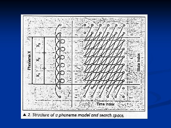
One-Pass DP Search Using a Linear Lexicon Linear lexicon n For three-word vocabulary , the search space： n

Maximum approximation： 　To assign each acoustic vector observed at time t to a (state, word) index pair. (s 1, w 1), …, (st, wt), …, (s. T, w. T) n

n n HMMs-the word interior (top) Word boundaries (bottom) Pr(w 1…wt)˙Pr(x 1…xt; s 1…st | w 1…wt) Note that the unknown word sequence and the unknown state sequence are determined simultaneously. ---DP algorithm

DP Recursion Two quantities: Q( t, s; w) score of the best path to time that ends in state s of word B( t, s ; w) start time of the best path up to time t tha t e nds in s ta te s of word w n DP solved that two types of transition rules for the path－ the word interior and word boundaries. n

In the word interior： 　Q(t, s; w) = max {P(xt, s | s’; w)˙Q(t-1, s’; w)} 　B(t, s; w) = B(t-1, smax(t, s; w) 　　Where smax(t, s; w) is the optimum predecessor state for the n hypothesis (t, s; w). n Word boundary： H(w; t) : = max {P(w|v)˙Q(t, Sv; v)}

The search procedure works with a timesynchronous breadth-first strategy. (table 2) n To reduce the storage requirements－ traceback array. n A strategy－Beam Search n

Table 2

One-Pass DP Search Using a three Lexicon To large-vocabulary recognition，for efficiency reasons－Using the form of a prefix tree n How to present the search algorithm for such a context ? ? n

n Structure the search space as follow: ( bigram )

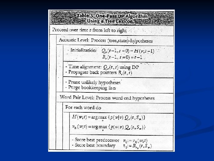
DP Recursion Qv (t, s) : = score of the best partial path that ends at time t in state s of the lexical tree for predecessor v. n Bv (t, s) : = start time of the best partial path that ends at time t in state s of the lexical tree for predecessor v. n

Qv(t, s) = max {P(wt, s | s’)˙Qv(t-1, s’)} n Bv(t, s) = Bv(t-1, svmax(t, s)) n Where svmax(t, s) is the optimum predecessor state for the hypothesis (t, s) and predecessor word v. n At the word boundaries H(w; t) : = max {P(w|v)˙Qv(t, Sw)} Qv(t-1, s=0) = H(v; t-1) Bv(t-1, s=0) = t-1

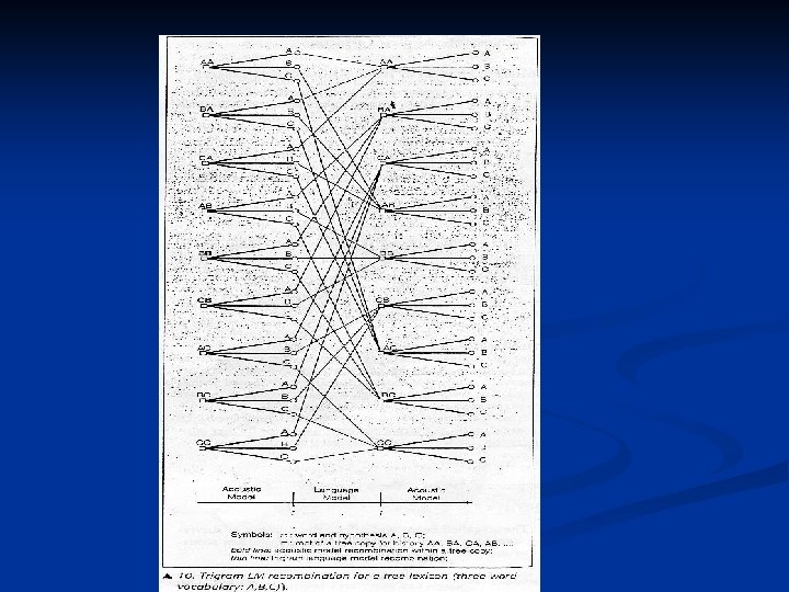
Extension to Trigram Language Models The root of each tree copy is labeled with its two-word history. n The probabilities or costs of each edge depend only on the edge itself. n Size of the potential search space is increased drastically. n Pruning strategy is even more crucial. n

Refinements and Implementation Issues n Pruning Refinements n Acoustic pruning： QAC(t) : = max{Qv(t, s)} Qv(t, s) < f. AC˙QAC(t) n Language model pruning (word end pruning) QLM(t) : = max{Qv(t, s=0)} Qv(t, s=0) < f. LM˙QLM(t) n Histogram pruning

Language Model Look-Ahead n To incorporate the language model probabilities as early as possible into the search process where W(s) is the set of words that can be reached from tree state s. n n n To incorporate the anticipated LM probabilities into the three pruning operations of the search Why? Reduce number of state hypotheses. Problem?

Fig. 11

Implementation n To arrive at an efficient implementation for tree search： n Set representation of active hypotheses n Set of active tree n Arc n Set of active HMM states (index s , score Q , back pointer) n Forward DP recombination (computational cost down) n Word boundaries、phoneme boundaries、HMM states n Direct access to each new successor hypotheses. n an exception－trigram LM.

Implementation n Traceback and Garbage Collection n Back pointer－>a special traceback array (word index, end time of the predecessor word, score, and back pointer) n Apply a garbage collection or purging method －> extend an additional component (time stamp)

n Table 4

One-Pass DP Search For Word Graph Construction Main idea：word alternative in regions of the speech signal. n To keep track of word sequence hypotheses whose scores are very to the optimal hypothesis, but don’t survive n To represents a word sequences by a word graph, Each word sequence should be close to single best sentence. n

Using the same principle of time synchrony for word graph: n =Conditional probability that word w produces the acoustic vectors n =Joint probability of observing the acoustic vector and a word sequence with end time t.

n decomposition－ where is probability of the language model => For construct a word graph，Introduce a formal definition of the word boundary

n Exploiting an m-gram language model we can recombine word sequence hypotheses at phrase level if they do not differ in their final (m-1) words. =>sufficient to distinguish partial word sequence hypotheses by their final words ∴ (included pruning strategy)

Word Pair Approximation n The crucial assumption now is that the dependence of the word boundary can be confined to the final word pair => or n Assuming the word pair approximation－ n n n At every time frame t, consider all word pairs =(v, w) For each triple(t ; v , w), keep track of word boundary 、word score At end of the speech signal word grapy is constructed by…. . .

n Fig 13

n How to computation ?

n table 5

n A third level－the phrase level Depending on whether the phrase-level recognition is carried out in a timesynchronous. Extended one-pass approach n Two-pass approach : cache-based language model n

n Fig 14

n Principal properties： There is a maximum for the number of incoming word edges in any node, namely the vocabulary size. n There is no maximum for the number of outgoing word edges. n n Two refinements of word graph method： Short words n Long words with identical ending portions may waste esearch effort. n

n table 6

n table 8