DYNAMIC PROGRAMMING Principle of optimality Coin changing problem

• DYNAMIC PROGRAMMING • • Principle of optimality Coin changing problem Computing a Binomial Coefficient Floyd’ algorithm Multi stage graph Optimal Binary Search Trees Knapsack Problem & Memory functions • GREEDY TECHNIQUE • • • Container loading problem Prim’s algorithm & Kruskal's Algorithm 0/1 Knapsack problem Optimal Merge pattern Huffman Trees

DYNAMIC PROGRAMMING • Dynamic programming is a technique for solving problems with overlapping • Rather than solving overlapping subproblems again and again, dynamic programming suggests solving each of the smaller subproblems only once and recording the results in a table from which a solution to the original problem can then be obtained • Since a majority of dynamic programming applications deal with optimization problems, we also need to mention a general principle that underlines such applications • Principle of optimality states that • An optimal solution to any instance of an optimization problem is composed of optimal solutions to its subinstances (or) • In an optimal sequence of decisions or choices, each subsequence must also be optimal

Coin Changing Problem • Give change for amount n using the minimum number of coins of denominations d 1<d 2 <. . . <dm. • Coin Changing Problem-1 • Coin Changing Problem-2

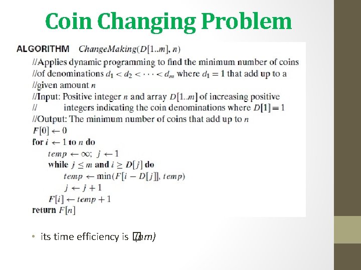
Coin Changing Problem • its time efficiency is � (nm)

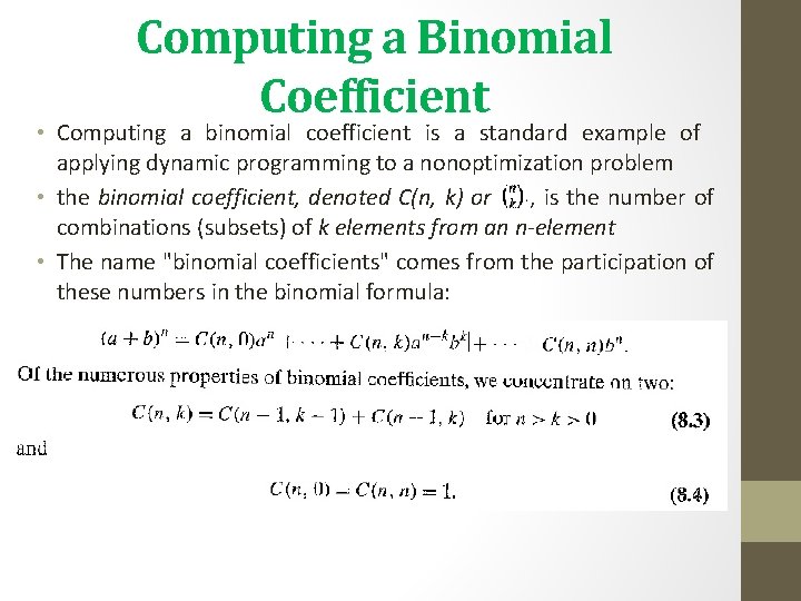
Computing a Binomial Coefficient • Computing a binomial coefficient is a standard example of applying dynamic programming to a nonoptimization problem • the binomial coefficient, denoted C(n, k) or , is the number of combinations (subsets) of k elements from an n-element • The name "binomial coefficients" comes from the participation of these numbers in the binomial formula:

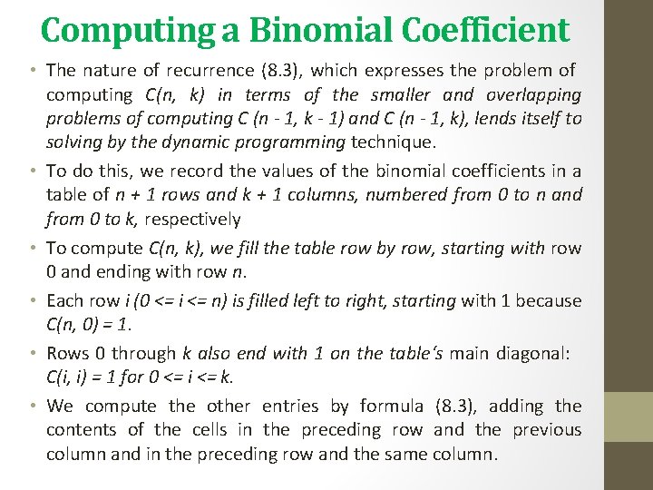
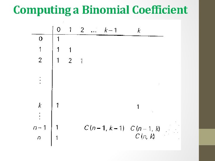
Computing a Binomial Coefficient • The nature of recurrence (8. 3), which expresses the problem of computing C(n, k) in terms of the smaller and overlapping problems of computing C (n - 1, k - 1) and C (n - 1, k), lends itself to solving by the dynamic programming technique. • To do this, we record the values of the binomial coefficients in a table of n + 1 rows and k + 1 columns, numbered from 0 to n and from 0 to k, respectively • To compute C(n, k), we fill the table row by row, starting with row 0 and ending with row n. • Each row i (0 <= i <= n) is filled left to right, starting with 1 because C(n, 0) = 1. • Rows 0 through k also end with 1 on the table‘s main diagonal: C(i, i) = 1 for 0 <= i <= k. • We compute the other entries by formula (8. 3), adding the contents of the cells in the preceding row and the previous column and in the preceding row and the same column.

Computing a Binomial Coefficient

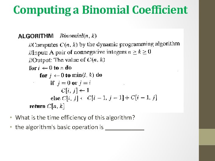
Computing a Binomial Coefficient • What is the time efficiency of this algorithm? • the algorithm's basic operation is ______

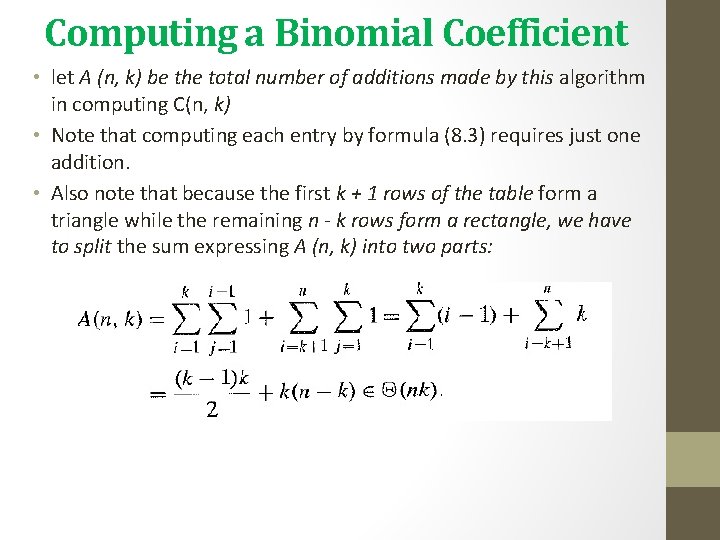
Computing a Binomial Coefficient • let A (n, k) be the total number of additions made by this algorithm in computing C(n, k) • Note that computing each entry by formula (8. 3) requires just one addition. • Also note that because the first k + 1 rows of the table form a triangle while the remaining n - k rows form a rectangle, we have to split the sum expressing A (n, k) into two parts:

Floyd’s Algorithm • It is called Floyd’s algorithm after its co-inventor Robert W. Floyd • Used to find solution for All-Pairs Shortest-Paths Problem • the all-pairs shortest paths problem asks to find the distances— i. e. , the lengths of the shortest paths— from each vertex to all other vertices • Application: pre computing distances for motion planning in computer games. • It is convenient to record the lengths of shortest paths in an n × n matrix D called the distance matrix: the element dij in the ith row and the jth column of this matrix indicates the length of the shortest path from the ith vertex to the jth vertex • It is applicable to both undirected and directed weighted graphs provided that they do not contain a cycle of a negative length

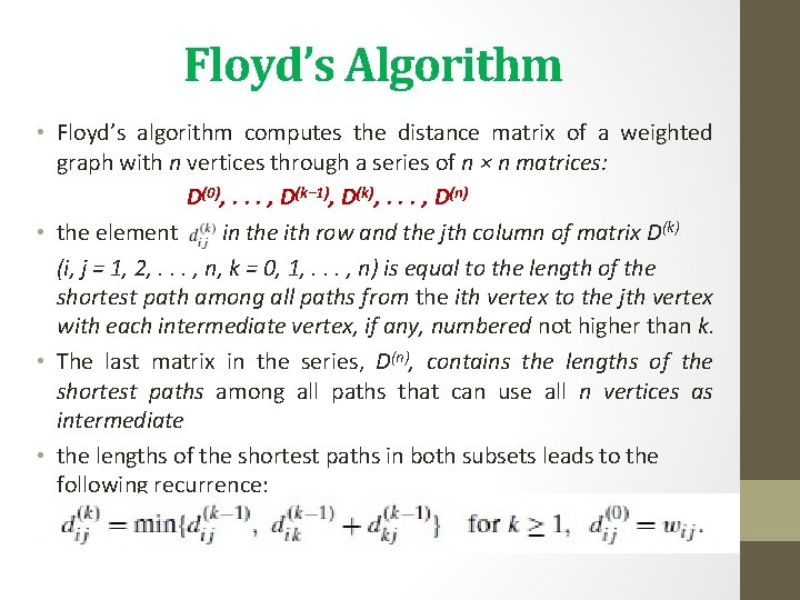
Floyd’s Algorithm • Floyd’s algorithm computes the distance matrix of a weighted graph with n vertices through a series of n × n matrices: D(0), . . . , D(k− 1), D(k), . . . , D(n) • the element in the ith row and the jth column of matrix D(k) (i, j = 1, 2, . . . , n, k = 0, 1, . . . , n) is equal to the length of the shortest path among all paths from the ith vertex to the jth vertex with each intermediate vertex, if any, numbered not higher than k. • The last matrix in the series, D(n), contains the lengths of the shortest paths among all paths that can use all n vertices as intermediate • the lengths of the shortest paths in both subsets leads to the following recurrence:

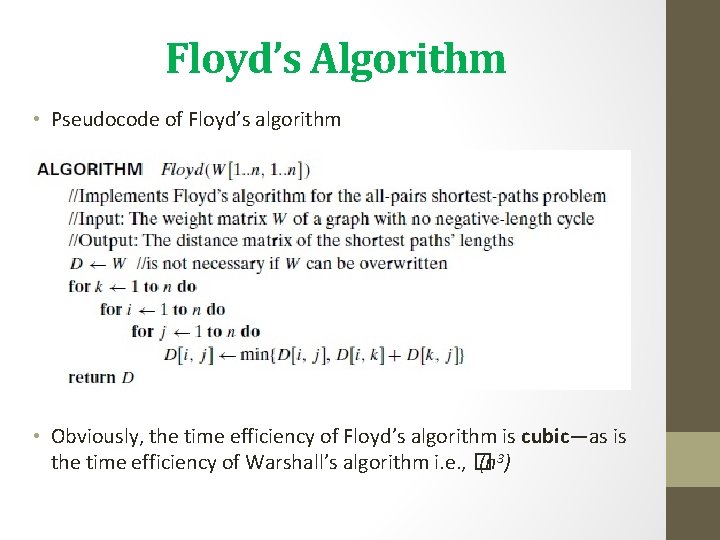
Floyd’s Algorithm • Pseudocode of Floyd’s algorithm • Obviously, the time efficiency of Floyd’s algorithm is cubic—as is the time efficiency of Warshall’s algorithm i. e. , � (n 3)

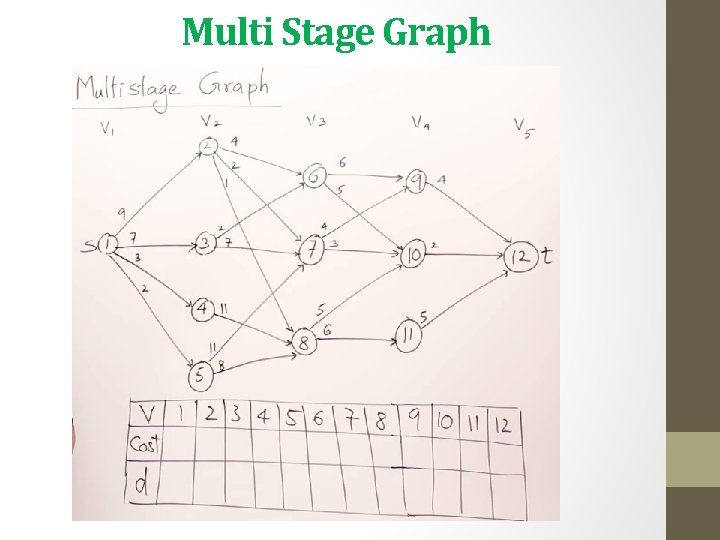
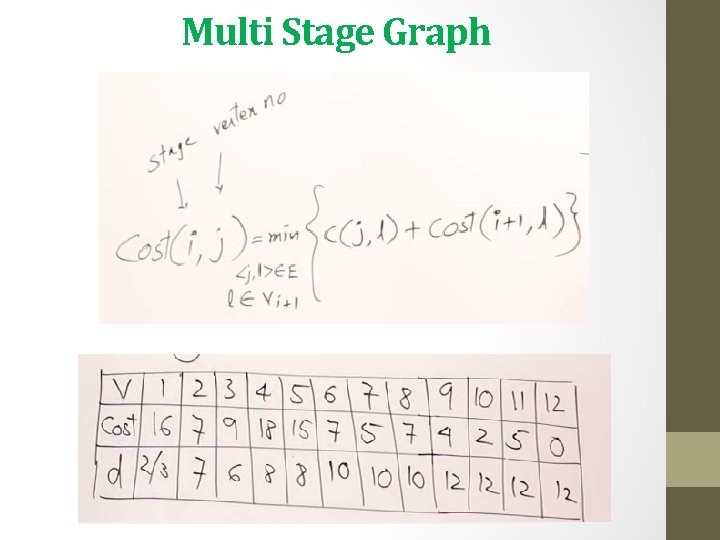
Multi Stage Graph

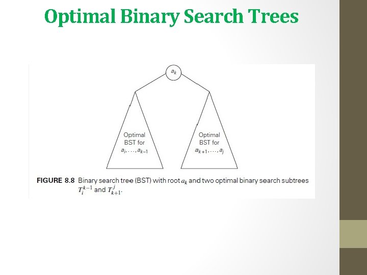
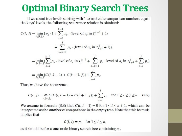
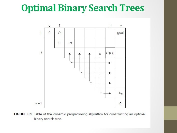
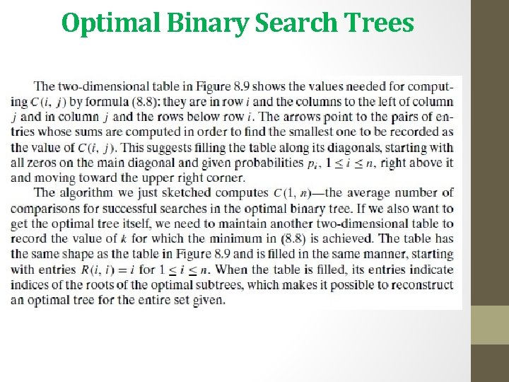
Optimal Binary Search Trees • A binary search tree is one of the most important data structures in computer science. • One of its principal applications is to implement a dictionary, a set of elements with the operations of searching, insertion, and deletion. • We limit our discussion to minimizing the average number of comparisons in a successful search. • As an example, consider four keys A, B, C, and D to be searched for with probabilities 0. 1, 0. 2, 0. 4, and 0. 3, respectively. • Figure 8. 7 depicts two out of 14 possible binary search trees containing these keys. • OBST - ABDUL BARI

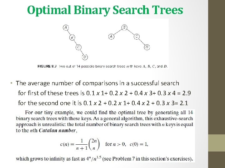
Optimal Binary Search Trees • The average number of comparisons in a successful search for first of these trees is 0. 1 x 1+ 0. 2 x 2 + 0. 4 x 3+ 0. 3 x 4 = 2. 9 for the second one it is 0. 1 x 2 + 0. 2 x 1+ 0. 4 x 2 + 0. 3 x 3= 2. 1

Optimal Binary Search Trees

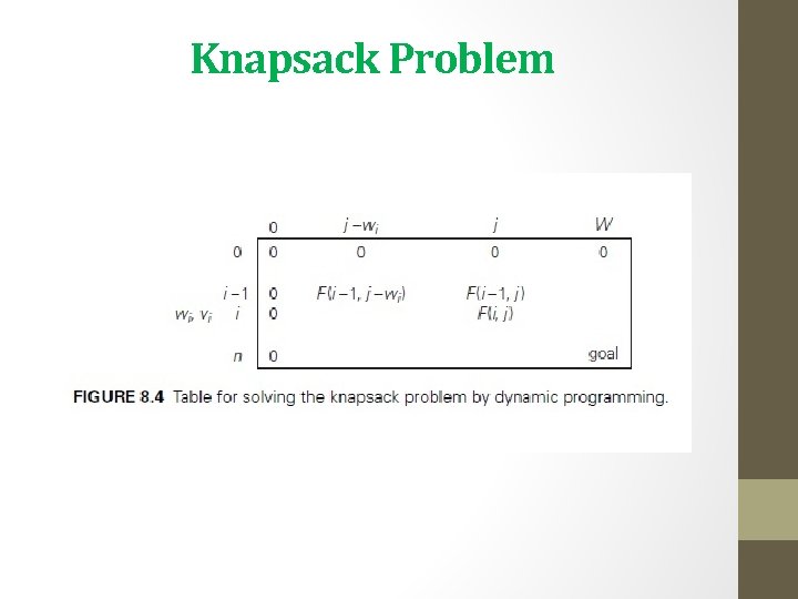
Knapsack Problem • KNAPSACK PROBLEM: Given n items of known weights w 1, . . . , wn and values v 1, . . . , vn and a knapsack of capacity W, find the most valuable subset of the items that fit into the knapsack • To design a dynamic programming algorithm, we need to derive a recurrence relation that expresses a solution to an instance of the knapsack problem in terms of solutions to its smaller subinstances • Let us consider an instance defined by the first i items, 1≤ i ≤ n, with weights w 1, . . . , wi, values v 1, . . . , vi , and knapsack capacity j, 1 ≤ j ≤ W. Let F(i, j) be the value of an optimal solution to this instance, i. e. , the value of the most valuable subset of the first i items that fit into the knapsack of capacity j. • We can divide all the subsets of the first i items that fit the knapsack of capacity j into two categories: those that do not include the ith item and those that do.

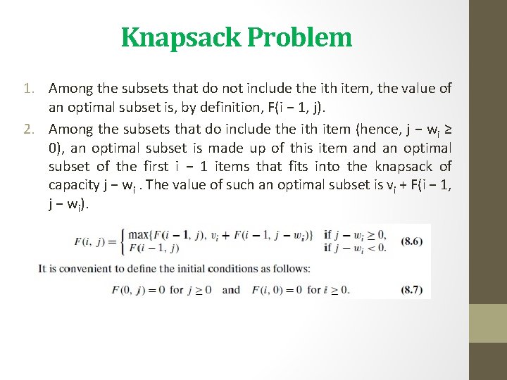
Knapsack Problem 1. Among the subsets that do not include the ith item, the value of an optimal subset is, by definition, F(i − 1, j). 2. Among the subsets that do include the ith item (hence, j − wi ≥ 0), an optimal subset is made up of this item and an optimal subset of the first i − 1 items that fits into the knapsack of capacity j − wi. The value of such an optimal subset is vi + F(i − 1, j − wi).

Knapsack Problem

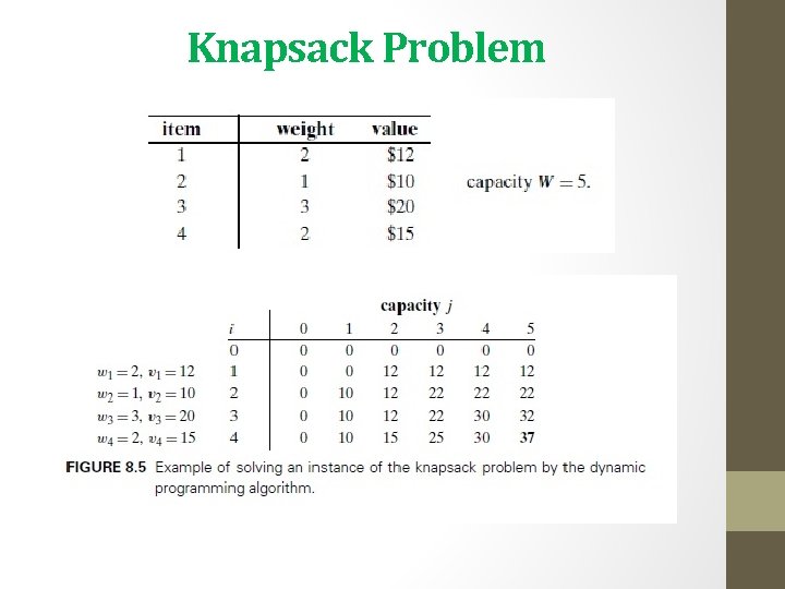
The Knapsack Problem • Thus, the maximal value is F(4, 5) = $37. We can find the composition of an optimal subset by back tracing the computations of this entry in the table. • Since F(4, 5) > F(3, 5), item 4 has to be included in an optimal solution along with an optimal subset for filling 5 − 2 = 3 remaining units of the knapsack capacity. • The value of the latter is F(3, 3). Since F(3, 3) = F(2, 3), item 3 need not be in an optimal subset. • Since F(2, 3) > F(1, 3), item 2 is a part of an optimal selection, which leaves element F(1, 3 − 1) to specify its remaining composition. • Similarly, since F(1, 2) > F(0, 2), item 1 is the final part of the optimal solution {item 1, item 2, item 4}. • The time efficiency and space efficiency of this algorithm are both in � (n. W). The time needed to find the composition of an optimal solution is in O(n).