Dynamic Programming Dynamic Programming algorithms address problems whose
Dynamic Programming • • Dynamic Programming algorithms address problems whose solution is recursive in nature, but has the following property: The direct implementation of the recursive solution results in identical recursive calls that are executed more than once. Dynamic programming implements such algorithms by evaluating the recurrence in a bottom-up manner, saving intermediate results that are later used in computing the desired solution 1
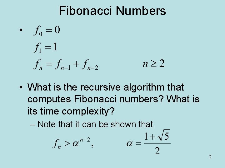
Fibonacci Numbers • • What is the recursive algorithm that computes Fibonacci numbers? What is its time complexity? – Note that it can be shown that 2
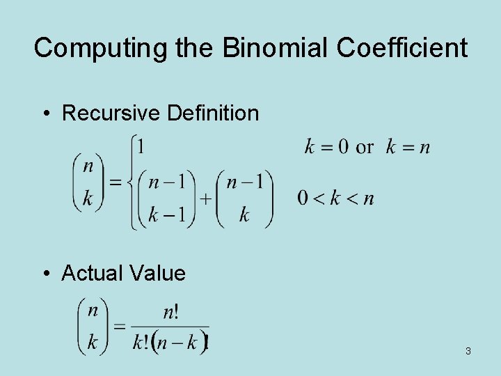
Computing the Binomial Coefficient • Recursive Definition • Actual Value 3
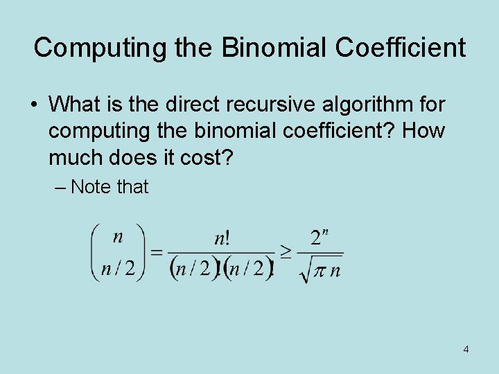
Computing the Binomial Coefficient • What is the direct recursive algorithm for computing the binomial coefficient? How much does it cost? – Note that 4

Dynamic Programming • Development of a dynamic programming solution to an optimization problem involves three steps 1. Characterize the structure of an optimal solution • Optimal substructures, where an optimal solution consists of sub-solutions that are optimal. • Overlapping sub-problems. 2. Recursively define the value of an optimal solution. 3. Compute the value of an optimal solution in a bottom-up manner. • Construct an optimal solution from the computed optimal value. 5
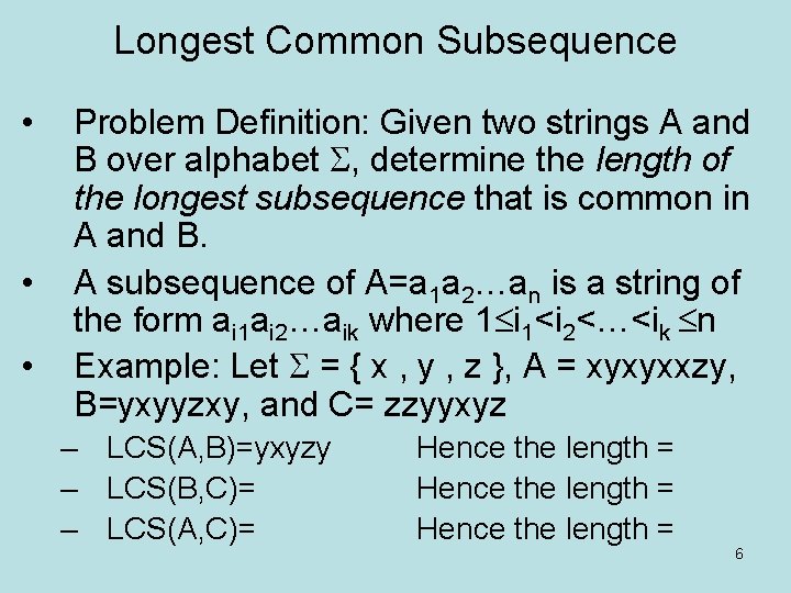
Longest Common Subsequence • • • Problem Definition: Given two strings A and B over alphabet , determine the length of the longest subsequence that is common in A and B. A subsequence of A=a 1 a 2…an is a string of the form ai 1 ai 2…aik where 1 i 1<i 2<…<ik n Example: Let = { x , y , z }, A = xyxyxxzy, B=yxyyzxy, and C= zzyyxyz – LCS(A, B)=yxyzy – LCS(B, C)= – LCS(A, C)= Hence the length = 6
Straight-Forward Solution • Brute-force search – How many subsequences exist in a string of length n? – How much time needed to check a string whether it is a subsequence of another string of length m? – What is the time complexity of the brute-force search algorithm of finding the length of the longest common subsequence of two strings of sizes n and m? 7
![Dynamic Programming Solution • Let L[i, j] denote the length of the longest common Dynamic Programming Solution • Let L[i, j] denote the length of the longest common](http://slidetodoc.com/presentation_image_h2/532abef7a6048ba72d16416cc9b901b9/image-8.jpg)
Dynamic Programming Solution • Let L[i, j] denote the length of the longest common subsequence of a 1 a 2…ai and b 1 b 2…bj, which are substrings of A and B of lengths n and m, respectively. Then L[i, j] = when i = 0 or j = 0 when i > 0, j > 0, ai=bj when i > 0, j > 0, ai bj 8
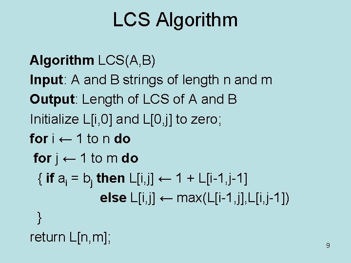
LCS Algorithm LCS(A, B) Input: A and B strings of length n and m Output: Length of LCS of A and B Initialize L[i, 0] and L[0, j] to zero; for i ← 1 to n do for j ← 1 to m do { if ai = bj then L[i, j] ← 1 + L[i-1, j-1] else L[i, j] ← max(L[i-1, j], L[i, j-1]) } return L[n, m]; 9
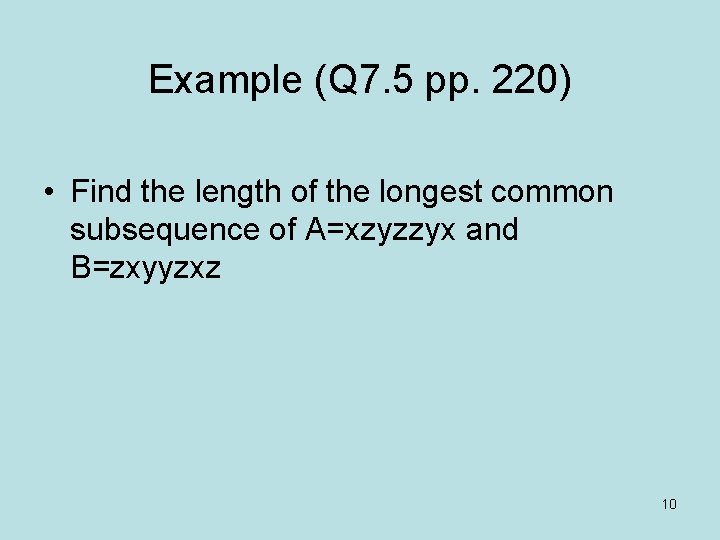
Example (Q 7. 5 pp. 220) • Find the length of the longest common subsequence of A=xzyzzyx and B=zxyyzxz 10
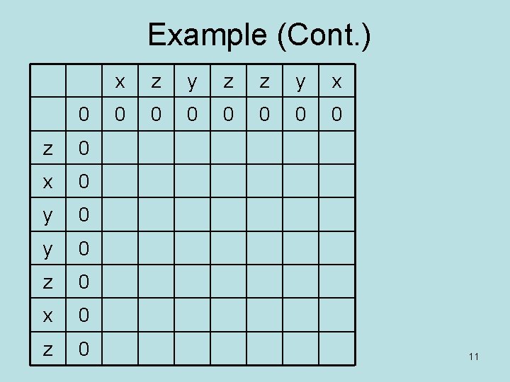
Example (Cont. ) 0 z 0 x 0 y 0 z 0 x z y z z y x 0 0 0 0 11
Complexity Analysis of LCS Algorithm • What is the time and space complexity of the algorithm? 12
Matrix Chain Multiplication • Assume Matrices A, B, and C have dimensions 2 10, 10 2, and 2 10 respectively. The number of scalar multiplications using the standard Matrix multiplication algorithm for – (A B) C is – A (B C) is • Problem Statement: Find the order of multiplying n matrices in which the number of scalar multiplications is minimum. 13
Straight-Forward Solution • Again, let us consider the brute-force method. We need to compute the number of different ways that we can parenthesize the product of n matrices. – e. g. how many different orderings do we have for the product of four matrices? – Let f(n) denote the number of ways to parenthesize the product M 1, M 2, …, Mn. • (M 1 M 2…Mk) (M k+1 M k+2…Mn) • What is f(2), f(3) and f(1)? 14
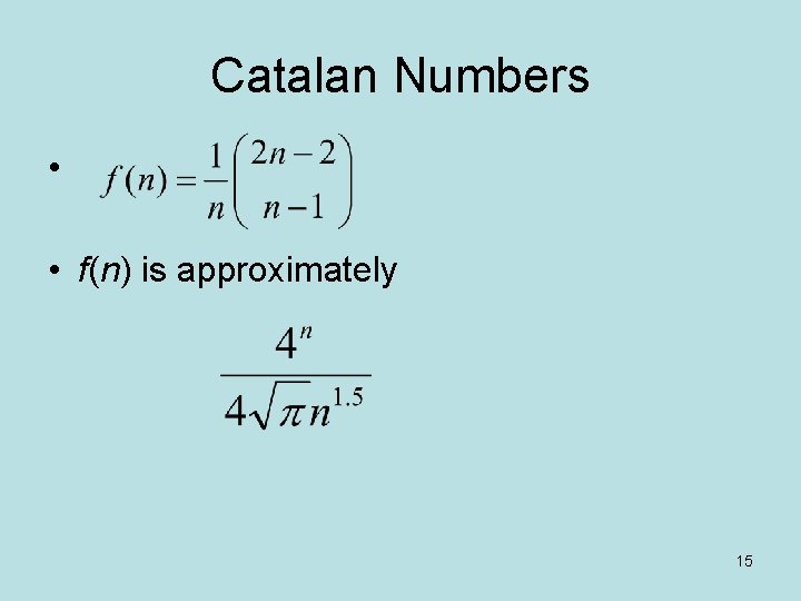
Catalan Numbers • • f(n) is approximately 15
Cost of Brute Force Method • How many possibilities do we have for parenthesizing n matrices? • How much does it cost to find the number of scalar multiplications for one parenthesized expression? • Therefore, the total cost is 16
The Recursive Solution • Since the number of columns of each matrix Mi is equal to the number of rows of Mi+1, we only need to specify the number of rows of all the matrices, plus the number of columns of the last matrix, r 1, r 2, …, rn+1 respectively. • Let the cost of multiplying the chain Mi…Mj (denoted by Mi, j) be C[i, j] • If k is an index between i+1 and j, what is the cost of multiplying Mi, j considering multiplying Mi, k-1 with Mk, j? • Therefore, C[1, n]= 17
![The Dynamic Programming Algorithm C[1, 1] C[1, 2] C[1, 3] C[1, 4] C[1, 5] The Dynamic Programming Algorithm C[1, 1] C[1, 2] C[1, 3] C[1, 4] C[1, 5]](http://slidetodoc.com/presentation_image_h2/532abef7a6048ba72d16416cc9b901b9/image-18.jpg)
The Dynamic Programming Algorithm C[1, 1] C[1, 2] C[1, 3] C[1, 4] C[1, 5] C[1, 6] C[2, 2] C[2, 3] C[2, 4] C[2, 5] C[2, 6] C[3, 3] C[3, 4] C[3, 5] C[3, 6] C[4, 4] C[4, 5] C[4, 6] C[5, 5] C[5, 6] C[6, 6] 18
![Mat. Chain Algorithm Mat. Chain Input: r[1. . n+1] of +ve integers (dimensions of Mat. Chain Algorithm Mat. Chain Input: r[1. . n+1] of +ve integers (dimensions of](http://slidetodoc.com/presentation_image_h2/532abef7a6048ba72d16416cc9b901b9/image-19.jpg)
Mat. Chain Algorithm Mat. Chain Input: r[1. . n+1] of +ve integers (dimensions of matr. ) Output: Least # of scalar multiplications required for i : = 1 to n do C[i, i] : = 0; // diagonal d 0 for d : = 1 to n-1 do // for diagonals d 1 to dn-1 for i : = 1 to n-d do { j : = i+d; C[i, j] : = ; for k : = i+1 to j do C[i, j] : = min{C[i, j], C[i, k-1]+C[k, j]+r[i]r[k]r[j+1]; }; return C[1, n]; 19
Example (Q 7. 11 pp. 221 -222) • Given as input 2 , 3 , 6 , 4 , 2 , 7 compute the minimum number of scalar multiplications: 20
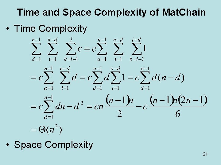
Time and Space Complexity of Mat. Chain • Time Complexity • Space Complexity 21
Assembly-Line Scheduling • Two parallel assembly lines in a factory, lines 1 and 2 • Each line has n stations Si, 1…Si, n • For each j, S 1, j does the same thing as S 2, j , but it may take a different amount of assembly time ai, j • Transferring away from line i after stage j costs ti, j • Also entry time ei and exit time xi at beginning and end 22
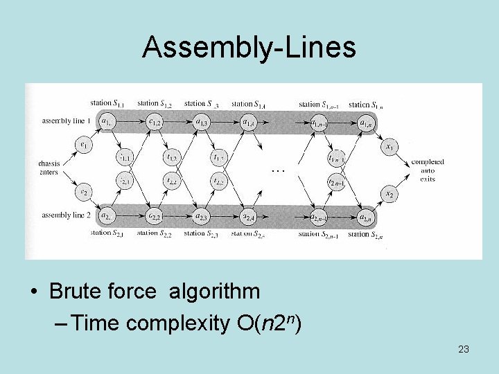
Assembly-Lines • Brute force algorithm – Time complexity O(n 2 n) 23
Finding Subproblem • Pick some convenient stage of the process – Say, just before the last station • What’s the next decision to make? – Whether the last station should be S 1, n or S 2, n • What do you need to know to decide which option is better? – What the fastest times are for S 1, n & S 2, n 24
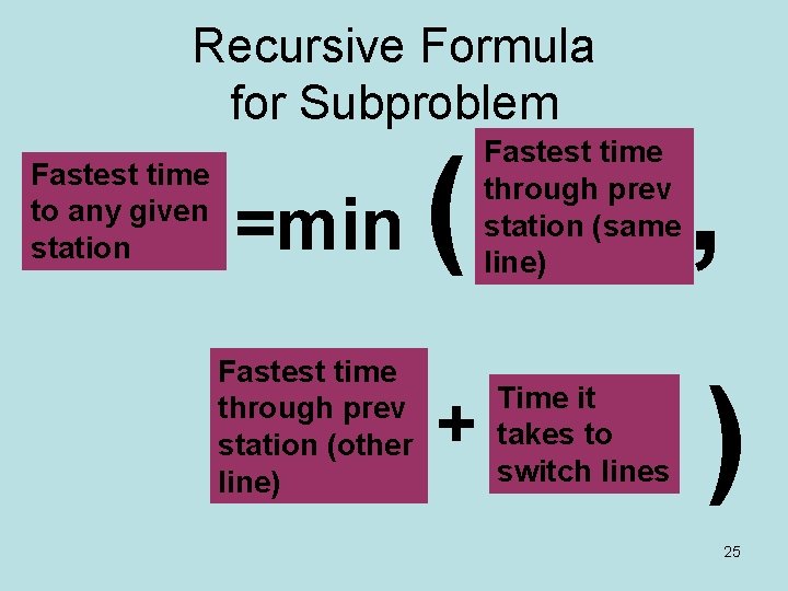
Recursive Formula for Subproblem Fastest time to any given station =min Fastest time through prev station (other line) ( + Fastest time through prev station (same line) Time it takes to switch lines , ) 25
![Recursive Formula (II) • Let fi [ j] denote the fastest possible time to Recursive Formula (II) • Let fi [ j] denote the fastest possible time to](http://slidetodoc.com/presentation_image_h2/532abef7a6048ba72d16416cc9b901b9/image-26.jpg)
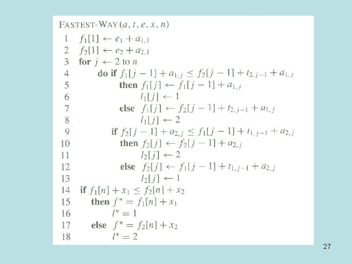
Recursive Formula (II) • Let fi [ j] denote the fastest possible time to get the chassis through S i, j • Have the following formulas: f 1[ 1] = e 1 + a 1, 1 f 1[ j] = min( f 1[ j-1] + a 1, j, f 2 [ j-1]+t 2, j-1+ a 1, j ) • Total time: f * = min( f 1[n] + x 1, f 2 [ n]+x 2) 26
27
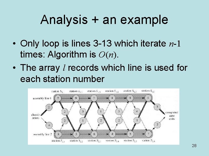
Analysis + an example • Only loop is lines 3 -13 which iterate n-1 times: Algorithm is O(n). • The array l records which line is used for each station number 28
All-Pairs Shortest Paths • Problem Statement: Let G = (V, E) be a directed graph in which each edge (i, j) has a nonnegative length l[i, j]. The allpairs shortest path problem is to find the length of the shortest path from each vertex to all other vertices. – The set of vertices V = {1, 2, …, n} – l[i, j] = if (i, j) E, i j. • Brute force algorithms? 29
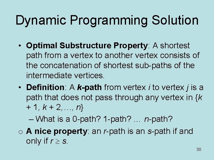
Dynamic Programming Solution • Optimal Substructure Property: A shortest path from a vertex to another vertex consists of the concatenation of shortest sub-paths of the intermediate vertices. • Definition: A k-path from vertex i to vertex j is a path that does not pass through any vertex in {k + 1, k + 2, …, n} – What is a 0 -path? 1 -path? … n-path? o A nice property: an r-path is an s-path if and only if r s. 30
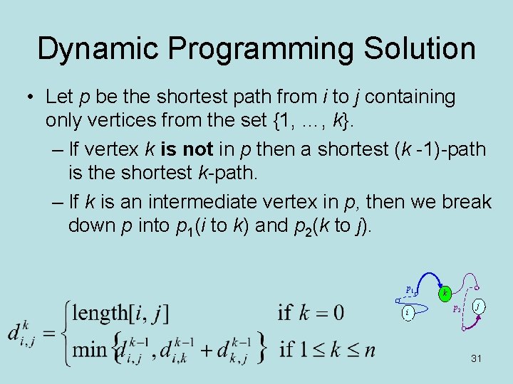
Dynamic Programming Solution • Let p be the shortest path from i to j containing only vertices from the set {1, …, k}. – If vertex k is not in p then a shortest (k -1)-path is the shortest k-path. – If k is an intermediate vertex in p, then we break down p into p 1(i to k) and p 2(k to j). p 1 i k p 2 j 31
![Floyd’s Algorithm Floyd Input: An n n matrix length[1. . n, 1. . n] Floyd’s Algorithm Floyd Input: An n n matrix length[1. . n, 1. . n]](http://slidetodoc.com/presentation_image_h2/532abef7a6048ba72d16416cc9b901b9/image-32.jpg)
Floyd’s Algorithm Floyd Input: An n n matrix length[1. . n, 1. . n] such that length[i, j] is the weight of the edge (i, j) in a directed graph G = ({1, 2, …, n}, E) Output: A matrix D with D[i, j] = [i, j] 1 D = length; //copy the input matrix length into D 2 for k = 1 to n do 3 for i = 1 to n do 4 for j = 1 to n do 5 D[i, j] = min{D[i, j] , D[i, k] + D[k, j]} 32
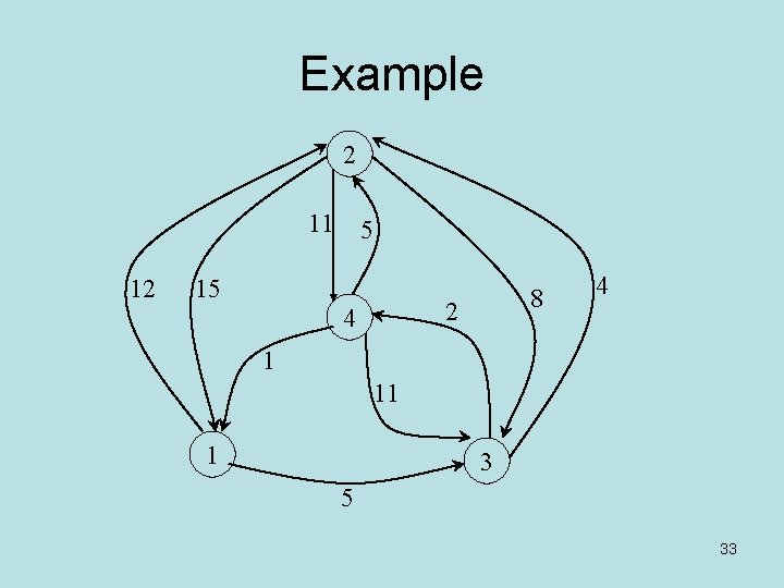
Example 2 11 5 12 15 8 2 4 4 1 11 1 3 5 33
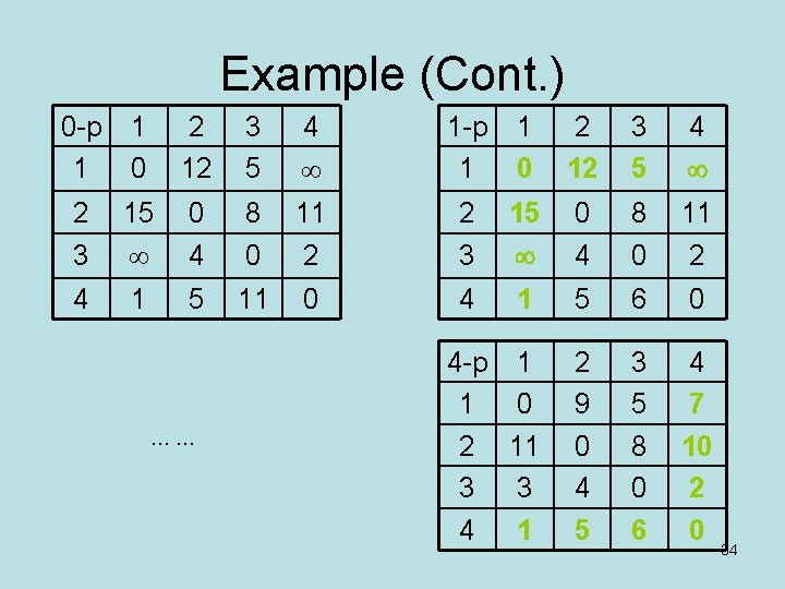
Example (Cont. ) 0 -p 1 1 0 2 12 3 5 4 1 -p 1 1 0 2 12 3 5 4 2 3 15 0 4 8 0 11 2 4 1 5 11 0 4 1 5 6 0 4 -p 1 1 0 2 11 3 3 4 1 2 9 0 4 5 3 5 8 0 6 4 7 10 2 0 …… 34
Time and Space Complexity • Time Complexity: • Space Complexity: 35
Greedy vs. DP Greedy: • Make a choice at each step. • Make the choice before solving the subproblems. • Solve top-down. Dynamic programming: • Make a choice at each step. • Choice depends on knowing optimal solutions to subproblems. Solve subproblems first. • Solve bottom-up. 36
Coin changing • Greedy algorithm works fine (for this example: [100, 25, 10, 5, 1]) – Prove greedy choice property – See Rosen (section 2. 1, pages 128, 129) • Greedy Method does not work in all cases – Coin sets = { 8, 5, 1} Change = 10. • Greedy Solution = {8, 1, 1} • Optimal Solution = { 5, 5} – What if Coin sets = {10, 6, 1}, Change = 12? 37
![Coin Changing: Dyn. Prog. 10 • A =12, denom = [10, 6, 1]? • Coin Changing: Dyn. Prog. 10 • A =12, denom = [10, 6, 1]? •](http://slidetodoc.com/presentation_image_h2/532abef7a6048ba72d16416cc9b901b9/image-38.jpg)
Coin Changing: Dyn. Prog. 10 • A =12, denom = [10, 6, 1]? • What could be the sub-problems? Described by which parameters? • How do we solve sub-problems? n n 6 1 How do we solve the trivial sub-problems? In which order do I have to solve subproblems? 38
0/1 Knapsack Problem • Greedy approach does not give optimal: – n = 3, W = 30 – weights = (20, 10, 5) – values = (180, 50) • Ratios = (180/20, 80/10, 50/5) = (9, 8, 10) • Greedy solution: (1, 0, 1) =180+50=230 • The optimal solution: (1, 1, 0) =180+80=260 39
0 -1 Knapsack problem: bruteforce approach Let’s first solve this problem with a straightforward algorithm • Since there are n items, there are 2 n possible combinations of items. • We go through all combinations and find the one with the most total value and with total weight less or equal to W • Running time will be O(2 n) 40
0 -1 Knapsack problem: bruteforce approach • Can we do better? • Yes, with an algorithm based on dynamic programming • We need to carefully identify the subproblems Let’s try this: If items are labeled 1. . n, then a subproblem would be to find an optimal solution for Sk = {items labeled 1, 2, . . k} 41
Defining a Subproblem If items are labeled 1. . n, then a subproblem would be to find an optimal solution for Sk = {items labeled 1, 2, . . k} • Let’s add another parameter: w, which will represent the exact weight for each subset of items • The subproblem is to compute B[k, w] 42
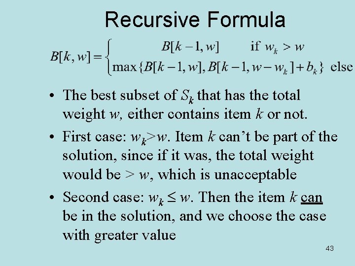
Recursive Formula • The best subset of Sk that has the total weight w, either contains item k or not. • First case: wk>w. Item k can’t be part of the solution, since if it was, the total weight would be > w, which is unacceptable • Second case: wk w. Then the item k can be in the solution, and we choose the case with greater value 43
![The 0/1 Knapsack Algorithm • B[k, w] = best selection from items 1 -k The 0/1 Knapsack Algorithm • B[k, w] = best selection from items 1 -k](http://slidetodoc.com/presentation_image_h2/532abef7a6048ba72d16416cc9b901b9/image-44.jpg)
The 0/1 Knapsack Algorithm • B[k, w] = best selection from items 1 -k with weight exactly equal to w • Base case: k = 0, no items to choose from. Total value is 0. • The answer will be the largest (rightmost) value in the last row (k = n) • Running time: O(n. W). • Note: not a polynomial-time algorithm if W is large 44
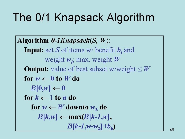
The 0/1 Knapsack Algorithm 0 -1 Knapsack(S, W): Input: set S of items w/ benefit bi and weight wi; max. weight W Output: value of best subset w/weight ≤ W for w 0 to W do B[0, w] 0 for k 1 to n do for w W downto wk do B[k, w] max(B[k-1, w], B[k-1, w-wk]+bk) 45
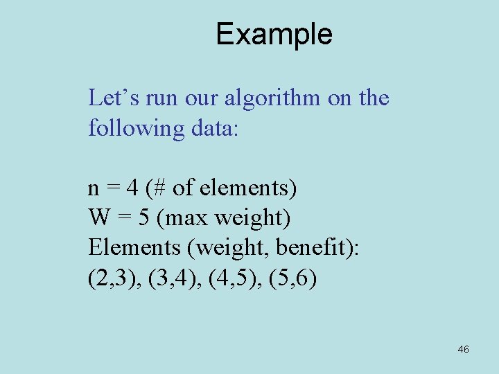
Example Let’s run our algorithm on the following data: n = 4 (# of elements) W = 5 (max weight) Elements (weight, benefit): (2, 3), (3, 4), (4, 5), (5, 6) 46
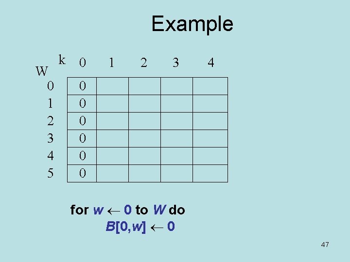
Example W 0 1 2 3 4 5 k 0 1 2 3 4 0 0 0 for w 0 to W do B[0, w] 0 47
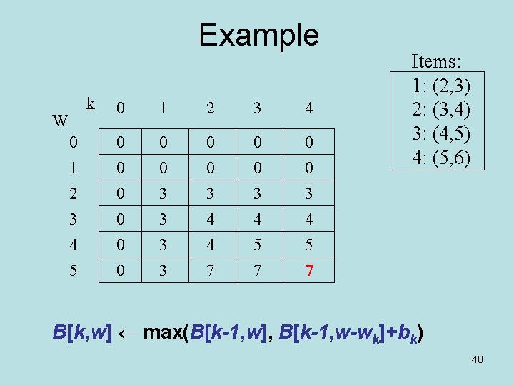
Example k W 0 1 2 3 4 5 0 1 2 3 4 0 0 0 0 3 3 0 0 3 4 4 7 0 0 3 4 5 7 Items: 1: (2, 3) 2: (3, 4) 3: (4, 5) 4: (5, 6) B[k, w] max(B[k-1, w], B[k-1, w-wk]+bk) 48
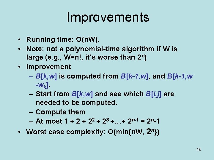
Improvements • Running time: O(n. W). • Note: not a polynomial-time algorithm if W is large (e. g. , W=n!, it’s worse than 2 n) • Improvement – B[k, w] is computed from B[k-1, w], and B[k-1, w -wk]. – Start from B[k, w] and see which B[i, j] are needed to be computed. – Compute them – At most 1 + 22 + 23 +…+ 2 n-1 = 2 n-1 • Worst case complexity: O(min{n. W, 2 n}) 49
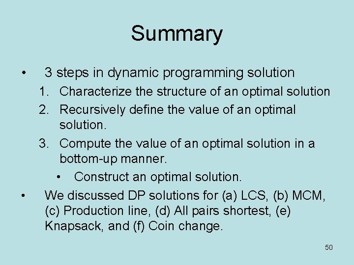
Summary • • 3 steps in dynamic programming solution 1. Characterize the structure of an optimal solution 2. Recursively define the value of an optimal solution. 3. Compute the value of an optimal solution in a bottom-up manner. • Construct an optimal solution. We discussed DP solutions for (a) LCS, (b) MCM, (c) Production line, (d) All pairs shortest, (e) Knapsack, and (f) Coin change. 50
- Slides: 50