Dynamic Programming Dr Benjamin Asubam Weyori Computer Science
Dynamic Programming Dr. Benjamin Asubam Weyori Computer Science & Informatics Department
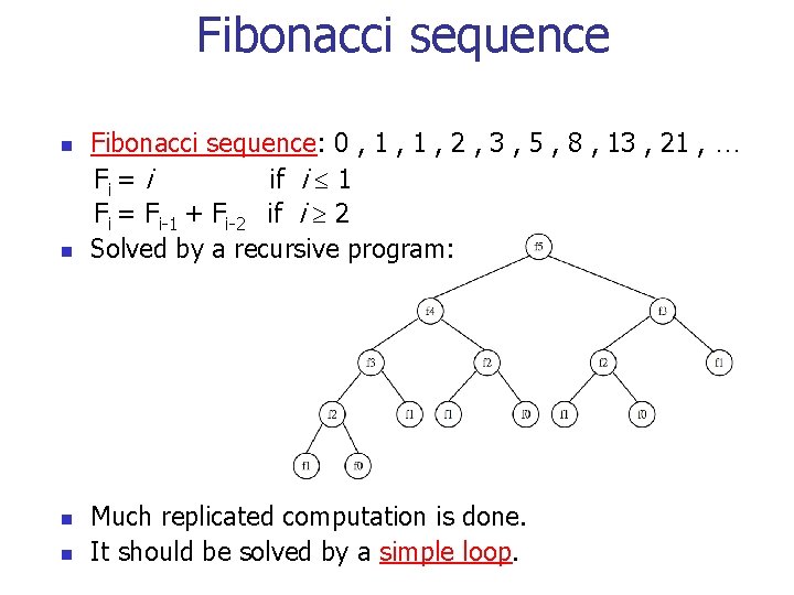
Fibonacci sequence n n Fibonacci sequence: 0 , 1 , 2 , 3 , 5 , 8 , 13 , 21 , … Fi = i if i 1 Fi = Fi-1 + Fi-2 if i 2 Solved by a recursive program: Much replicated computation is done. It should be solved by a simple loop.
Dynamic Programming n Dynamic Programming is an algorithm design method that can be used when the solution to a problem may be viewed as the result of a sequence of decisions
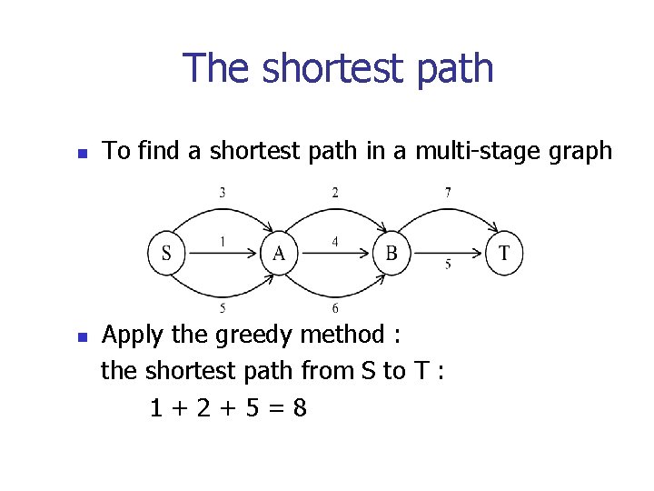
The shortest path n n To find a shortest path in a multi-stage graph Apply the greedy method : the shortest path from S to T : 1+2+5=8
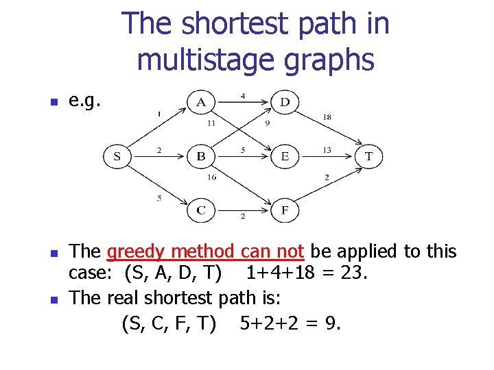
The shortest path in multistage graphs n n n e. g. The greedy method can not be applied to this case: (S, A, D, T) 1+4+18 = 23. The real shortest path is: (S, C, F, T) 5+2+2 = 9.
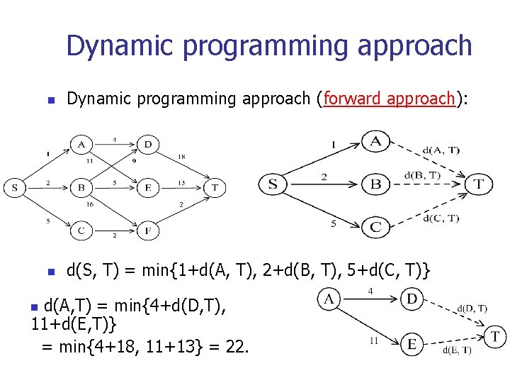
Dynamic programming approach n Dynamic programming approach (forward approach): n d(S, T) = min{1+d(A, T), 2+d(B, T), 5+d(C, T)} d(A, T) = min{4+d(D, T), 11+d(E, T)} = min{4+18, 11+13} = 22. n
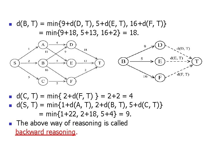
n n d(B, T) = min{9+d(D, T), 5+d(E, T), 16+d(F, T)} = min{9+18, 5+13, 16+2} = 18. d(C, T) = min{ 2+d(F, T) } = 2+2 = 4 d(S, T) = min{1+d(A, T), 2+d(B, T), 5+d(C, T)} = min{1+22, 2+18, 5+4} = 9. The above way of reasoning is called backward reasoning.
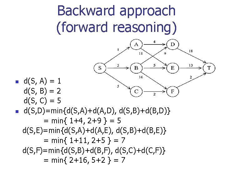
Backward approach (forward reasoning) n n d(S, A) = 1 d(S, B) = 2 d(S, C) = 5 d(S, D)=min{d(S, A)+d(A, D), d(S, B)+d(B, D)} = min{ 1+4, 2+9 } = 5 d(S, E)=min{d(S, A)+d(A, E), d(S, B)+d(B, E)} = min{ 1+11, 2+5 } = 7 d(S, F)=min{d(S, B)+d(B, F), d(S, C)+d(C, F)} = min{ 2+16, 5+2 } = 7
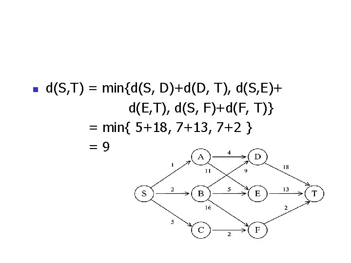
n d(S, T) = min{d(S, D)+d(D, T), d(S, E)+ d(E, T), d(S, F)+d(F, T)} = min{ 5+18, 7+13, 7+2 } =9
Principle of optimality n n n Principle of optimality: Suppose that in solving a problem, we have to make a sequence of decisions D 1, D 2, …, Dn. If this sequence is optimal, then the last k decisions, 1 k n must be optimal. e. g. the shortest path problem If i, i 1, i 2, …, j is a shortest path from i to j, then i 1, i 2, …, j must be a shortest path from i 1 to j In summary, if a problem can be described by a multistage graph, then it can be solved by dynamic programming.

Dynamic programming n Forward approach and backward approach: n n n Note that if the recurrence relations are formulated using the forward approach then the relations are solved backwards. i. e. , beginning with the last decision On the other hand if the relations are formulated using the backward approach, they are solved forwards. To solve a problem by using dynamic programming: n n Find out the recurrence relations. Represent the problem by a multistage graph.
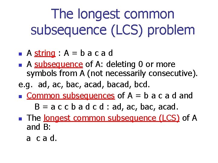
The longest common subsequence (LCS) problem A string : A = b a c a d n A subsequence of A: deleting 0 or more symbols from A (not necessarily consecutive). e. g. ad, ac, bac, acad, bcd. n Common subsequences of A = b a c a d and B = a c c b a d c d : ad, ac, bac, acad. n The longest common subsequence (LCS) of A and B: a c a d. n
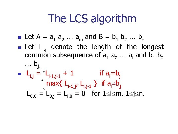
The LCS algorithm n n n Let A = a 1 a 2 am and B = b 1 b 2 bn Let Li, j denote the length of the longest common subsequence of a 1 a 2 ai and b 1 b 2 bj. Li, j = Li-1, j-1 + 1 if ai=bj max{ Li-1, j, Li, j-1 } if ai bj L 0, 0 = L 0, j = Li, 0 = 0 for 1 i m, 1 j n.
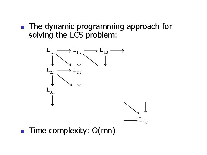
n n The dynamic programming approach for solving the LCS problem: Time complexity: O(mn)
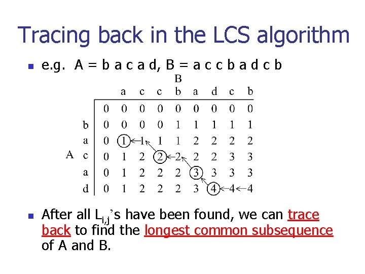
Tracing back in the LCS algorithm n n e. g. A = b a c a d, B = a c c b a d c b After all Li, j’s have been found, we can trace back to find the longest common subsequence of A and B.
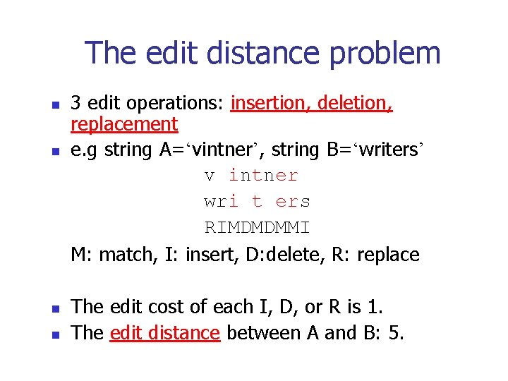
The edit distance problem n n 3 edit operations: insertion, deletion, replacement e. g string A=‘vintner’, string B=‘writers’ v intner wri t ers RIMDMDMMI M: match, I: insert, D: delete, R: replace The edit cost of each I, D, or R is 1. The edit distance between A and B: 5.
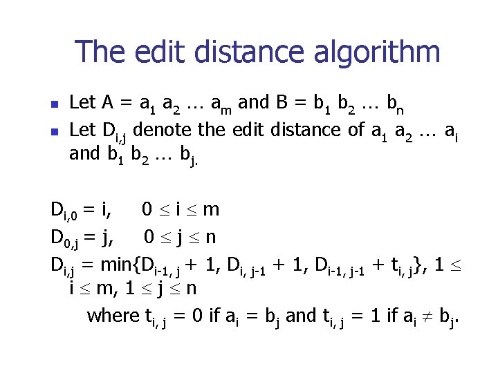
The edit distance algorithm n n Let A = a 1 a 2 am and B = b 1 b 2 bn Let Di, j denote the edit distance of a 1 a 2 ai and b 1 b 2 bj. Di, 0 = i, 0 i m D 0, j = j, 0 j n Di, j = min{Di-1, j + 1, Di, j-1 + 1, Di-1, j-1 + ti, j}, 1 i m, 1 j n where ti, j = 0 if ai = bj and ti, j = 1 if ai bj.
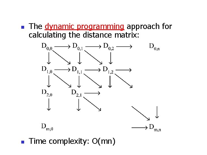
n n The dynamic programming approach for calculating the distance matrix: Time complexity: O(mn)
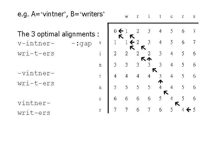
e. g. A=‘vintner’, B=‘writers’ The 3 optimal alignments : v-intner-: gap wri-t-ers -vintnerwri-t-ers vintnerwrit-ers
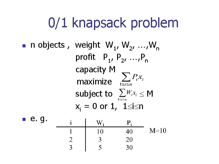
0/1 knapsack problem n n n objects , weight W 1, W 2, , Wn profit P 1, P 2, , Pn capacity M maximize subject to M xi = 0 or 1, 1 i n e. g.
The multistage graph solution n The 0/1 knapsack problem can be described by a multistage graph.
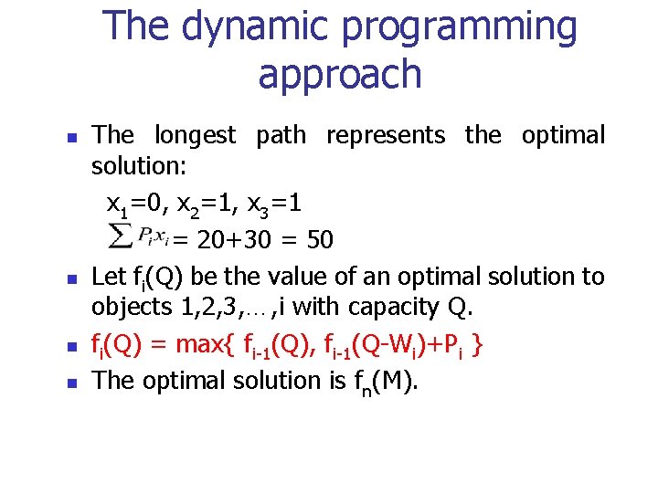
The dynamic programming approach n n The longest path represents the optimal solution: x 1=0, x 2=1, x 3=1 = 20+30 = 50 Let fi(Q) be the value of an optimal solution to objects 1, 2, 3, …, i with capacity Q. fi(Q) = max{ fi-1(Q), fi-1(Q-Wi)+Pi } The optimal solution is fn(M).
Optimal binary search trees n e. g. binary search trees for 3, 7, 9, 12;
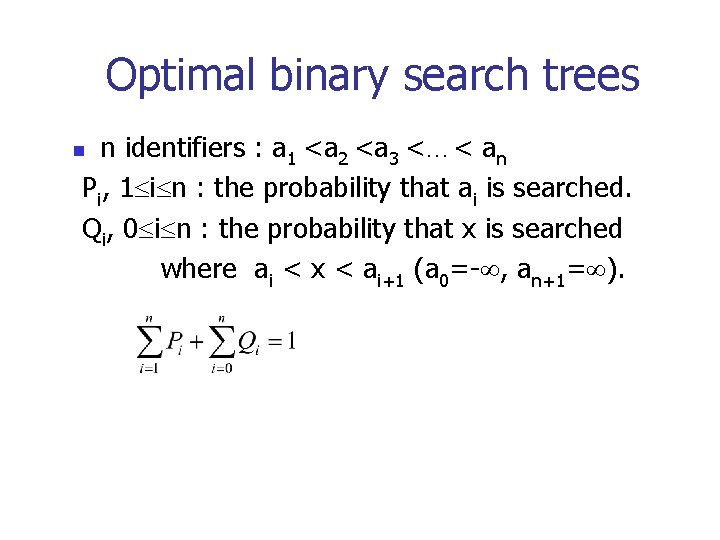
Optimal binary search trees n identifiers : a 1 <a 2 <a 3 <…< an Pi, 1 i n : the probability that ai is searched. Qi, 0 i n : the probability that x is searched where ai < x < ai+1 (a 0=- , an+1= ). n
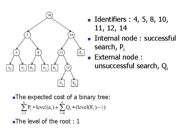
n n n Identifiers : 4, 5, 8, 10, 11, 12, 14 Internal node : successful search, Pi External node : unsuccessful search, Qi n The expected cost of a binary tree: n The level of the root : 1
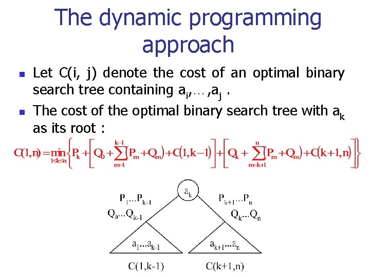
The dynamic programming approach n n Let C(i, j) denote the cost of an optimal binary search tree containing ai, …, aj. The cost of the optimal binary search tree with ak as its root :
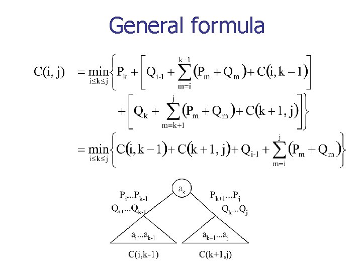
General formula
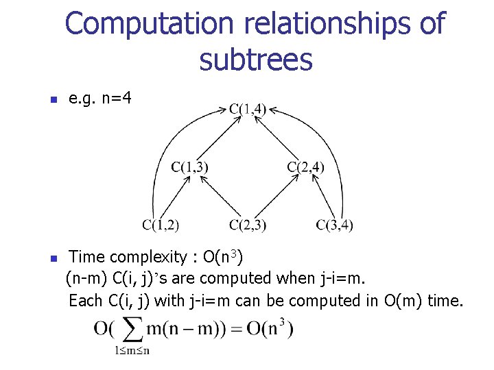
Computation relationships of subtrees n n e. g. n=4 Time complexity : O(n 3) (n-m) C(i, j)’s are computed when j-i=m. Each C(i, j) with j-i=m can be computed in O(m) time.
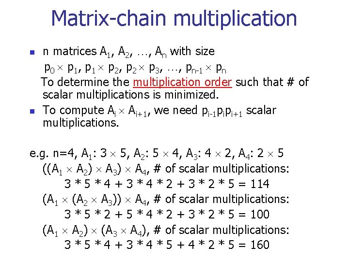
Matrix-chain multiplication n matrices A 1, A 2, …, An with size p 0 p 1, p 1 p 2, p 2 p 3, …, pn-1 pn To determine the multiplication order such that # of scalar multiplications is minimized. To compute Ai Ai+1, we need pi-1 pipi+1 scalar multiplications. e. g. n=4, A 1: 3 5, A 2: 5 4, A 3: 4 2, A 4: 2 5 ((A 1 A 2) A 3) A 4, # of scalar multiplications: 3 * 5 * 4 + 3 * 4 * 2 + 3 * 2 * 5 = 114 (A 1 (A 2 A 3)) A 4, # of scalar multiplications: 3 * 5 * 2 + 5 * 4 * 2 + 3 * 2 * 5 = 100 (A 1 A 2) (A 3 A 4), # of scalar multiplications: 3 * 5 * 4 + 3 * 4 * 5 + 4 * 2 * 5 = 160
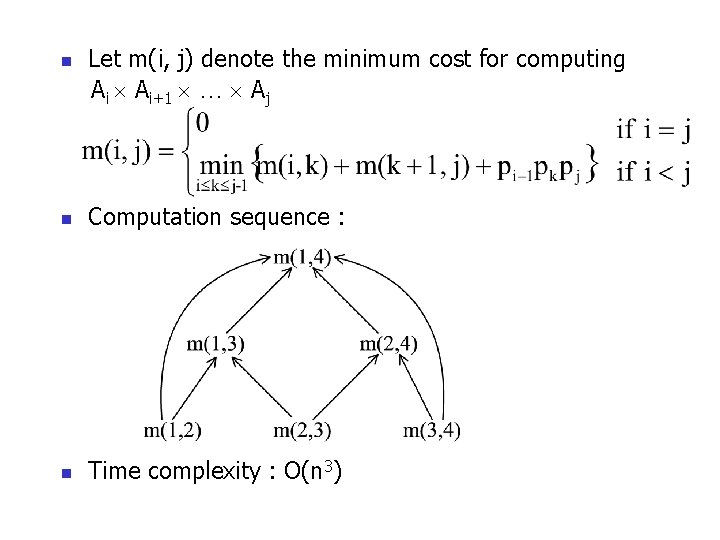
n Let m(i, j) denote the minimum cost for computing Ai Ai+1 … Aj n Computation sequence : n Time complexity : O(n 3)
Minimum Spanning Trees

Carolina Challenge
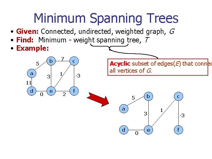
Minimum Spanning Trees • Given: Connected, undirected, weighted graph, G • Find: Minimum - weight spanning tree, T • Example: b 5 a 3 7 c 1 -3 Acyclic subset of edges(E) that connec all vertices of G. 11 d 0 e 2 f b 5 a d 3 0 e c 1 -3 f
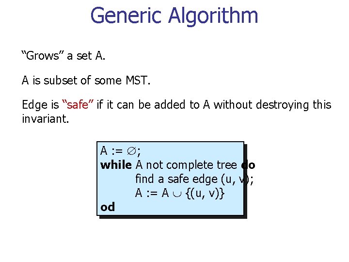
Generic Algorithm “Grows” a set A. A is subset of some MST. Edge is “safe” if it can be added to A without destroying this invariant. A : = ; while A not complete tree do find a safe edge (u, v); A : = A {(u, v)} od
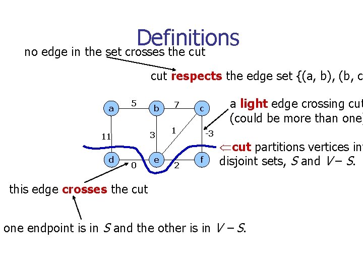
Definitions no edge in the set crosses the cut respects the edge set {(a, b), (b, c a 5 3 11 d b 0 e 7 1 2 a light edge crossing cut (could be more than one) c -3 f Ücut partitions vertices int disjoint sets, S and V – S. this edge crosses the cut one endpoint is in S and the other is in V – S.
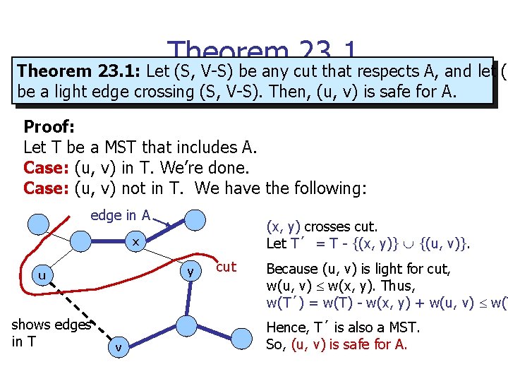
Theorem 23. 1: Let (S, V-S) be any cut that respects A, and let (u be a light edge crossing (S, V-S). Then, (u, v) is safe for A. Proof: Let T be a MST that includes A. Case: (u, v) in T. We’re done. Case: (u, v) not in T. We have the following: edge in A (x, y) crosses cut. Let T´ = T - {(x, y)} {(u, v)}. x y u shows edges in T v cut Because (u, v) is light for cut, w(u, v) w(x, y). Thus, w(T´) = w(T) - w(x, y) + w(u, v) w(T Hence, T´ is also a MST. So, (u, v) is safe for A.
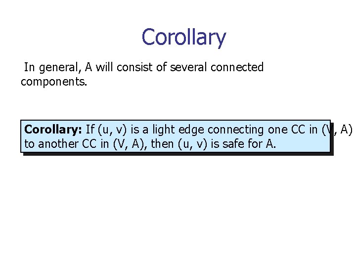
Corollary In general, A will consist of several connected components. Corollary: If (u, v) is a light edge connecting one CC in (V, A) to another CC in (V, A), then (u, v) is safe for A.
Kruskal’s Algorithm n n Starts with each vertex in its own component. Repeatedly merges two components into one by choosing a light edge that connects them (i. e. , a light edge crossing the cut between them). Scans the set of edges in monotonically increasing order by weight. Uses a disjoint-set data structure to determine whether an edge connects vertices in different components.
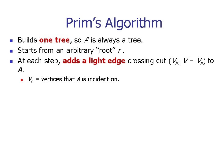
Prim’s Algorithm n n n Builds one tree, so A is always a tree. Starts from an arbitrary “root” r. At each step, adds a light edge crossing cut (VA, V - VA) to A. n VA = vertices that A is incident on.
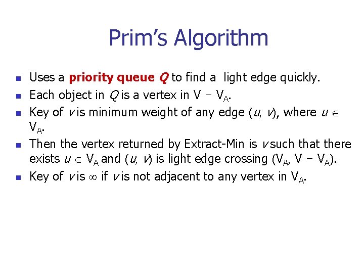
Prim’s Algorithm n n n Uses a priority queue Q to find a light edge quickly. Each object in Q is a vertex in V - VA. Key of v is minimum weight of any edge (u, v), where u V A. Then the vertex returned by Extract-Min is v such that there exists u VA and (u, v) is light edge crossing (VA, V - VA). Key of v is if v is not adjacent to any vertex in VA.
![Prim’s Algorithm Q : = V[G]; Complexity: for each u Q do Using binary Prim’s Algorithm Q : = V[G]; Complexity: for each u Q do Using binary](http://slidetodoc.com/presentation_image_h2/043326ab31b588396c7f79f1c96061fb/image-41.jpg)
Prim’s Algorithm Q : = V[G]; Complexity: for each u Q do Using binary heaps: O(E lg V). key[u] : = Initialization – O(V). od; Building initial queue – O(V). key[r] : = 0; V Extract-Min’s – O(V lg. V). [r] : = NIL; E Decrease-Key’s – O(E lg V). while Q do u : = Extract - Min(Q); Using Fibonacci heaps: O(E + V lg V). for each v Adj[u] do if v Q w(u, v) < key[v] then (see book) [v] : = u; key[v] : = w(u, v) decrease-key operation fi od od Note: A = {(v, [v]) : v v - {r} - Q}.
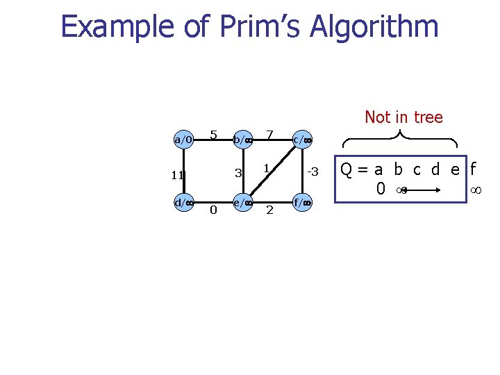
Example of Prim’s Algorithm Not in tree a/0 5 3 11 d/ b/ 0 e/ 7 1 2 c/ -3 f/ Q=a b c d e f 0
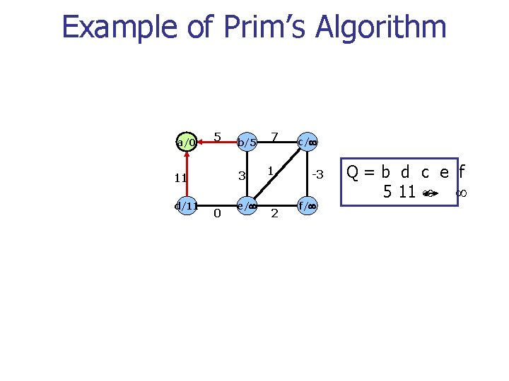
Example of Prim’s Algorithm a/0 5 3 11 d/11 b/5 0 e/ 7 1 2 c/ -3 f/ Q=b d c e f 5 11
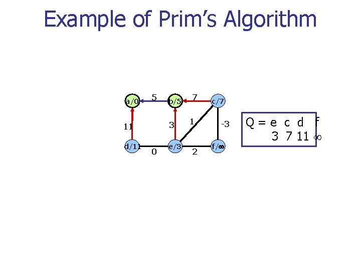
Example of Prim’s Algorithm a/0 5 3 11 d/11 b/5 0 e/3 7 1 2 c/7 -3 f/ Q=e c d f 3 7 11
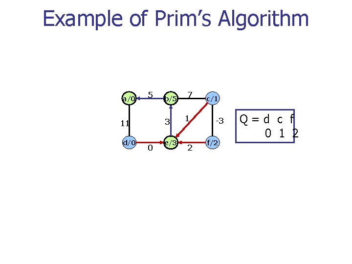
Example of Prim’s Algorithm a/0 5 3 11 d/0 b/5 0 e/3 7 1 2 c/1 -3 f/2 Q=d c f 0 1 2
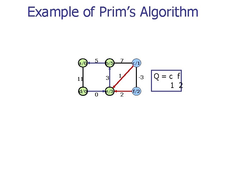
Example of Prim’s Algorithm a/0 5 3 11 d/0 b/5 0 e/3 7 1 2 c/1 -3 f/2 Q=c f 1 2
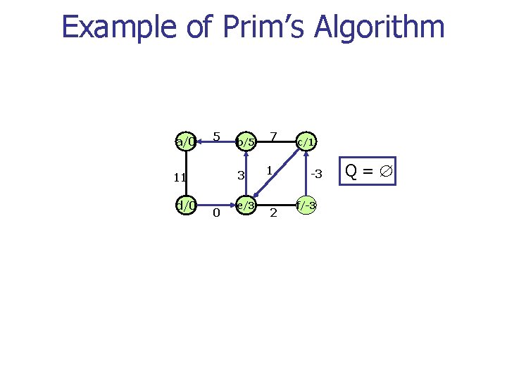
Example of Prim’s Algorithm a/0 5 3 11 d/0 b/5 0 e/3 7 1 2 c/1 -3 f/-3 Q=
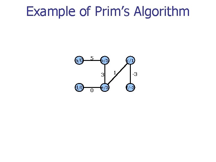
Example of Prim’s Algorithm a/0 5 b/5 3 d/0 0 e/3 c/1 1 -3 f/-3
- Slides: 48