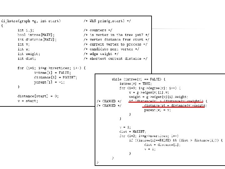
Dynamic Programming Dijkstras Algorithm n Goal Find the

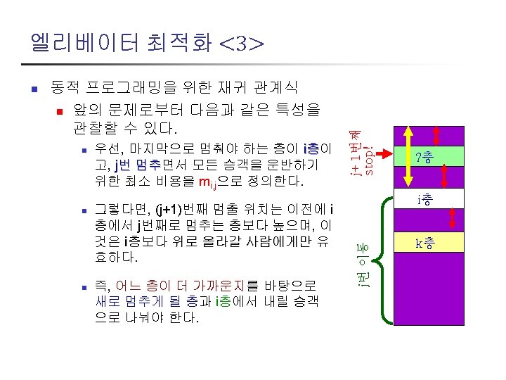
Dynamic Programming

Dijkstra’s Algorithm n Goal: Find the shortest path from s to t 24 2 9 s 3 18 14 6 30 15 11 5 5 16 20 7 6 2 44 4 19 6 t

S={ } PQ = { s, 2, 3, 4, 5, 6, 7, t } 0 24 2 9 s 14 18 2 6 30 15 11 5 5 16 20 7 3 44 6 4 19 6 t

S={s} PQ = { 2, 3, 4, 5, 6, 7, t } X 9 0 24 2 9 s 18 X 14 14 2 6 30 15 11 5 5 16 20 7 X 15 3 44 6 4 19 6 t

S={s} PQ = { 2, 3, 4, 5, 6, 7, t } X 9 0 24 2 9 s 18 X 14 14 2 6 30 15 11 5 5 16 20 7 X 15 3 44 6 4 19 6 t

S = { s, 2 } PQ = { 3, 4, 5, 6, 7, t } X 9 0 24 2 9 s 18 X 14 14 2 6 30 15 11 5 5 16 20 7 X 15 3 44 6 4 19 6 t

S = { s, 2 } PQ = { 3, 4, 5, 6, 7, t } X 33 X 9 0 24 2 9 s 18 X 14 14 2 6 30 15 5 11 5 16 20 7 X 15 3 44 6 4 19 6 t

S = { s, 2, 6 } PQ = { 3, 4, 5, 7, t } 32 X 33 X X 9 0 24 2 9 s 18 X 14 14 2 6 30 15 44 X 11 5 5 16 20 7 X 15 3 44 6 4 19 6 t

S = { s, 2, 6, 7 } PQ = { 3, 4, 5, t } 32 X 33 X X 9 0 24 2 9 s 18 X 14 14 2 6 30 15 X 35 44 X 5 5 X 15 11 16 20 7 3 44 6 4 19 6 t 59 X

S = { s, 2, 3, 6, 7 } PQ = { 4, 5, t } 32 X X 9 0 24 2 9 s 18 X 14 14 2 6 30 15 35 X 5 5 X 15 11 16 20 7 3 44 6 4 19 6 t 51 X X

S = { s, 2, 3, 5, 6, 7 } PQ = { 4, t } 32 X 9 0 24 2 9 s 1 6 4 18 X 14 15 2 30 34 5 5 1 5 X 11 16 20 7 3 44 45 X 6 4 19 6 t 50

S = { s, 2, 3, 4, 5, 6, 7 } PQ = { t } 32 X 9 0 24 2 9 s 18 X 14 14 2 6 30 15 34 5 5 X 15 11 16 20 7 3 44 4 X 4 5 6 19 6 t 50

Dynamic Programming In mathematics and computer science, dynamic programming is a method of solving complex problems by breaking them down into simpler steps - wikipedia

Algorithms Review n Backtracking n n Greedy Algorithm n n search every possible solution optimal guaranteed inefficient find the best at each stage – MST not always optimal needs a proof Dynamic Programming n efficient recursive algorithm

Recursive Algorithm n Divide-and-Conquor n n n top-down solution Fibonnaci can be inefficient duplicated computations F(n) = F(n-1) + F(n-2) = {F(n-2)+F(n-3)} + {F(n-3)+F(n-4)} = [{F(n-3)+F(n-4)}+{F(n-4)+F(n-5)}] +[{F(n-4)+F(n-5)}+{F(n-5)+F(n-6)}] =. . . Dynamic Programming n n n bottom-up recursive and solve above limitations Fibonacci n n calculate F(1), F(2), . . and store the results use them to calculate F(n)

Binomial Coefficient n k = n-1 k-1 + k int bino(int n, int k) { if (k==0 || n==k) return 1; else return bino(n-1, k-1) + bino(n-1, k); } {bino(n-2, k-2) + bino(n-2, k-1)} + {bino(n-2, k-1) + bino(n-2, k)} Redundancy !

Binomial Coefficient (2) k. C 0 = k. Ck = 1 1 2 C 1 = 1 C 0 + 1 C 1 1 1 3 C 1 = 2 C 0 + 2 C 1 3 C 2 = 2 C 1 + 2 C 2 1 4 C 1 = 3 C 0 + 3 C 1 1 3 3 1 4 C 2 = 3 C 1 + 3 C 2 1 4 6 4 1 . . . bino(int n, int k) { long bc[n][k]; for( int i=0; i<=n; i++) for( int j=0; j<=min(i, k); j++ ) if( j==0 || j==I ) bc[i][j]=1; else bc[i][j] = bc[i-1][j-1] + bc[i-1][j]; return bc[n][k]; }

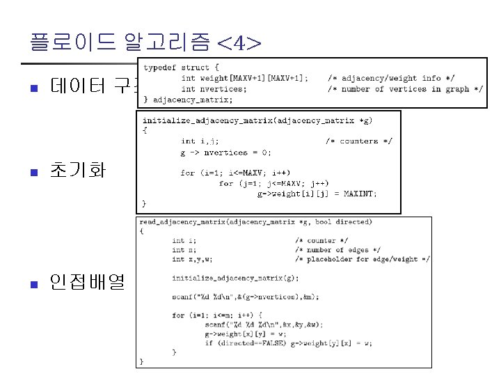
Floyd’s Algorithm n find all pairs shortest paths n n n Floyd Alg. n n apply Dijkstra alg. for each vertex inefficient number each vertex from 1 to n start from W(0)=W, ends with W(n) which is a set of shortest paths – bottom up compute W(k) from W(k-1) - recursion typical dynamic programming problem

Floyd’s Algorithm n Adjacent Matrix: W 1 v 1 3 5 v 5 3 n 9 1 v 4 v 2 3 2 4 v 3 W(k)[i][j] n n shortest path from vi to vj the path traverses vertices among {v 1, v 2, . . . , vk}

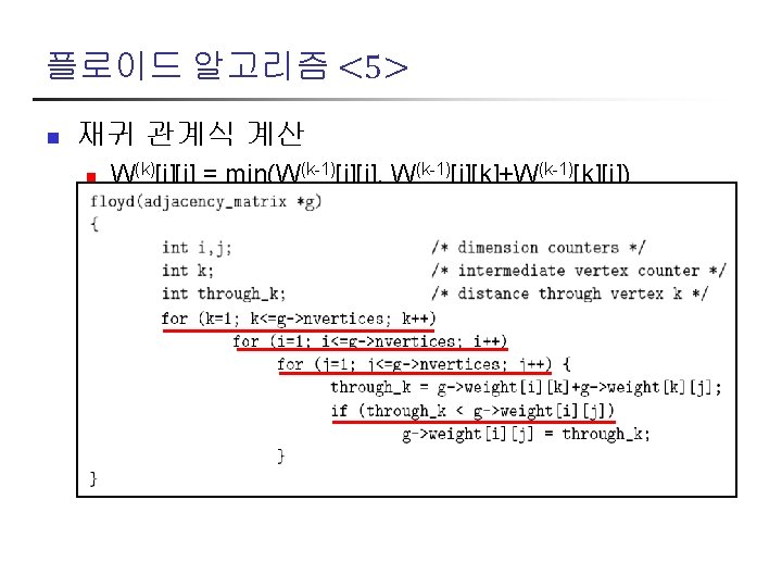
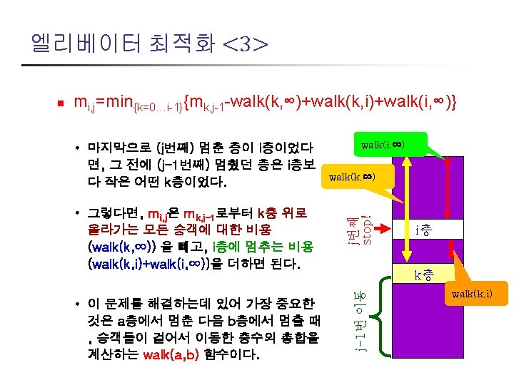
Floyd’s Algorithm n W(k)[i][j] = min(W(k-1)[i][j], W(k-1)[i][k]+W(k-1)[k][j]) Case 1 n n n Case 2 shortest path from vi to vj using {v 1, v 2, … , vk} Case 1: the path does not visit vk (5) (4) n Ex) W [1][3] = 3 Case 2: the path visits vk (2) (1) n Ex) W [5][3] = W [5][2] + W [2][3] = 4+3 = 7