Dynamic Programming CSE 3318 Algorithms and Data Structures

Dynamic Programming CSE 3318 – Algorithms and Data Structures University of Texas at Arlington Alexandra Stefan (Includes images, formulas and examples from CLRS, Dr. Bob Weems, wikipedia) 3/2/2021 1

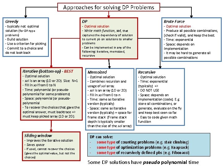
Approaches for solving DP Problems Greedy DP problems) captures the dependency of solution to current pb on solutions to smaller problems - Can be implemented in any of the following: iterative, memoized, recursive - typically not optimal solution (for DP-type - Build solution - Use a criterion for picking - Commit to a choice and do not look back Iterative (bottom-up) - BEST - Optimal solution - sol is an array (1 D or 2 D). Size: N+1 - Fill in sol from 0 to N - Time: polynomial (or pseudopolynomial for some problems) - Space: polynomial (or pseudopolynomial - To recover the choices that gave the optimal answer, must backtrace => must keep picked array (1 D or 2 D). Sliding window - Improves the iterative solution - Saves space - If used, cannot recover the choices (gives the optimal value, but not the choices) Brute Force - Optimal solution - Write math function, sol, that Memoized - Optimal solution - Combines recursion and usage of sol array. - sol is an array (1 D or 2 D) - Fill in sol from 0 to n - Time: same as iterative version (typically) - Space: same as iterative version (typically) + space for frame stack. (Frame stack depth is typically smaller than the size of the sol array) - Optimal solution - Produce all possible combinations, [check if valid], and keep the best. - Time: exponential - Space: depends on implementation - It may be hard to generate all possible combinations Recursive - Optimal solution - Time: exponential (typically) => - DO NOT USE - Space: depends on implementation (code). E. g. store all combinations, or generate, evaluate on the fly and keep best seen so far. - Easy to code given math function DP can solve: - some type of counting problems (e. g. stair climbing) - some type of optimization problems (e. g. Knapsack) - some type of recursively defined pbs (e. g. Fibonacci) Some DP solutions have pseudo polynomial time

Dynamic Programming (DP) - CLRS • Dynamic programming (DP) applies when a problem has both of these properties: 1. Optimal substructure: “optimal solutions to a problem incorporate optimal solutions to related subproblems, which we may solve independently”. 2. Overlapping subproblems: “a recursive algorithm revisits the same problem repeatedly”. • Dynamic programming is typically used to: – Solve optimization problems that have the above properties. – Solve counting problems –e. g. Stair Climbing or Matrix Traversal. – Speed up existing recursive implementations of problems that have overlapping subproblems (property 2) – e. g. Fibonacci. • Compare dynamic programming with divide and conquer. 3

Iterative or Bottom-Up Dynamic Programming • Main type of solution for DP problems • We can define the problems size and solve problems from size 0 going up to the size we need. • Iterative – because it uses a loop • Bottom-up because you solve problems from the bottom (the smallest problem size) up to the original problem size. 4

Bottom-Up vs. Top Down • There are two versions of dynamic programming. – Bottom-up. – Top-down (or memoization). • Bottom-up: – Iterative, solves problems in sequence, from smaller to bigger. • Top-down: – Recursive, start from the larger problem, solve smaller problems as needed. – For any problem that we solve, store the solution, so we never have to compute the same solution twice. – This approach is also called memoization. 5

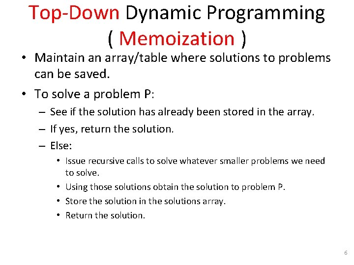
Top-Down Dynamic Programming ( Memoization ) • Maintain an array/table where solutions to problems can be saved. • To solve a problem P: – See if the solution has already been stored in the array. – If yes, return the solution. – Else: • Issue recursive calls to solve whatever smaller problems we need to solve. • Using those solutions obtain the solution to problem P. • Store the solution in the solutions array. • Return the solution. 6

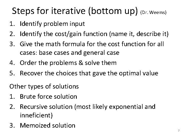
Steps for iterative (bottom up) (Dr. Weems) 1. Identify problem input 2. Identify the cost/gain function (name it, describe it) 3. Give the math formula for the cost function for all cases: base cases and general case 4. Order the problems & solve them 5. Recover the choices that gave the optimal value Other types of solutions 1. Brute force solution 2. Recursive solution (most likely exponential and inneficient) 3. Memoized solution 7

Weighted Interval Scheduling (Job Scheduling) 8

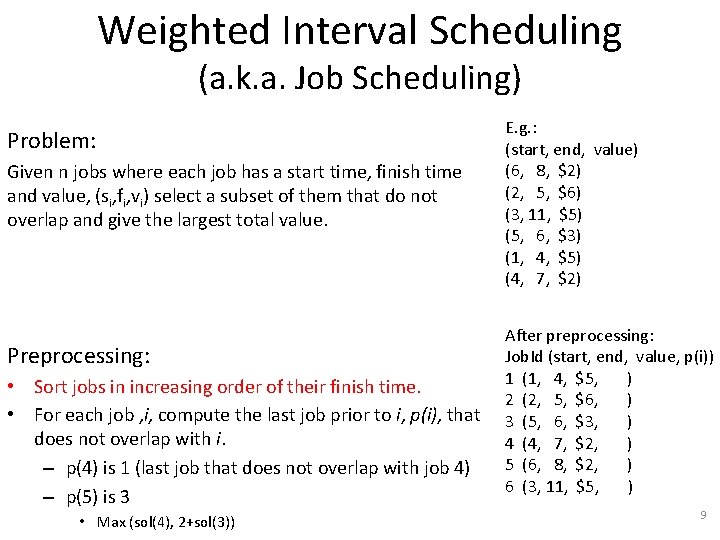
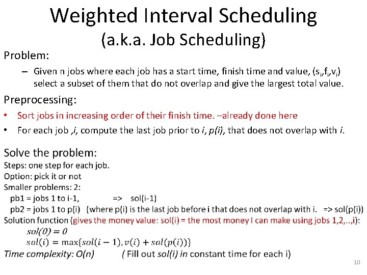
Weighted Interval Scheduling (a. k. a. Job Scheduling) Problem: Given n jobs where each job has a start time, finish time and value, (si, fi, vi) select a subset of them that do not overlap and give the largest total value. Preprocessing: • Sort jobs in increasing order of their finish time. • For each job , i, compute the last job prior to i, p(i), that does not overlap with i. – p(4) is 1 (last job that does not overlap with job 4) – p(5) is 3 • Max (sol(4), 2+sol(3)) E. g. : (start, end, value) (6, 8, $2) (2, 5, $6) (3, 11, $5) (5, 6, $3) (1, 4, $5) (4, 7, $2) After preprocessing: Job. Id (start, end, value, p(i)) 1 (1, 4, $5, ) 2 (2, 5, $6, ) 3 (5, 6, $3, ) 4 (4, 7, $2, ) 5 (6, 8, $2, ) 6 (3, 11, $5, ) 9

Weighted Interval Scheduling Problem: (a. k. a. Job Scheduling) – Given n jobs where each job has a start time, finish time and value, (si, fi, vi) select a subset of them that do not overlap and give the largest total value. Preprocessing: • Sort jobs in increasing order of their finish time. –already done here • For each job , i, compute the last job prior to i, p(i), that does not overlap with i. 10

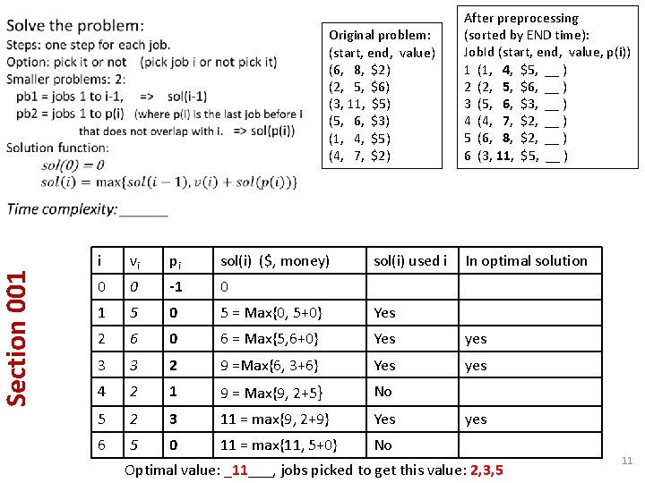
Section 001 Original problem: (start, end, value) (6, 8, $2) (2, 5, $6) (3, 11, $5) (5, 6, $3) (1, 4, $5) (4, 7, $2) sol(i) used i After preprocessing (sorted by END time): Job. Id (start, end, value, p(i)) 1 (1, 4, $5, __ ) 2 (2, 5, $6, __ ) 3 (5, 6, $3, __ ) 4 (4, 7, $2, __ ) 5 (6, 8, $2, __ ) 6 (3, 11, $5, __ ) i vi pi sol(i) ($, money) In optimal solution 0 0 -1 0 1 5 0 5 = Max{0, 5+0} Yes 2 6 0 6 = Max{5, 6+0} Yes yes 3 3 2 9 =Max{6, 3+6} Yes yes 4 2 1 9 = Max{9, 2+5} No 5 2 3 11 = max{9, 2+9} Yes 6 5 0 11 = max{11, 5+0} No yes Optimal value: _11___, jobs picked to get this value: 2, 3, 5 11

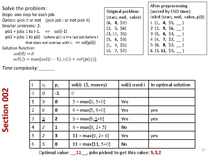
Section 002 Original problem: (start, end, value) (6, 8, $2) (2, 5, $6) (3, 11, $5) (5, 6, $3) (1, 4, $5) (4, 7, $2) sol(i) used i After preprocessing (sorted by END time): Job. Id (start, end, value, p(i)) 1 (1, 4, $5, __ ) 2 (2, 5, $6, __ ) 3 (5, 6, $3, __ ) 4 (4, 7, $2, __ ) 5 (6, 8, $2, __ ) 6 (3, 11, $5, __ ) i vi pi sol(i) ($, money) In optimal solution 0 0 -1 0 1 5 0 5 = max{0, 5+0} Yes 2 6 0 6 = max{5, 6+0} Yes yes 3 3 2 9 = max{6, 3+6} Yes yes 4 2 1 9 = max{9, 2+ 5} No 5 2 3 11 = max{9, 2+ 9} Yes 6 5 0 11 = max{11, 5+0} No yes Optimal value: __11__, jobs picked to get this value: 5, 3, 2 12

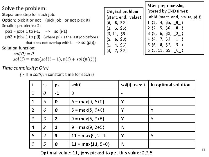
Original problem: (start, end, value) (6, 8, $2) (2, 5, $6) (3, 11, $5) (5, 6, $3) (1, 4, $5) (4, 7, $2) After preprocessing (sorted by END time): Job. Id (start, end, value, p(i)) 1 (1, 4, $5, _0_ ) 2 (2, 5, $6, _0_ ) 3 (5, 6, $3, _2_ ) 4 (4, 7, $2, _1_ ) 5 (6, 8, $2, _3_ ) 6 (3, 11, $5, _0_ ) i vi pi sol(i) used i In optimal solution 0 0 -1 0 - 1 5 0 5 = max{0, 5+0} Y 2 6 0 6 = max{5, 6+0} Y Y 3 3 2 9 = max{6, 3+6} Y Y 4 2 1 9 = max{9, 2+5} N 5 2 3 11 = max{9, 2+9} Y 6 5 0 11 = max{11, 5+0} N Y Optimal value: 11, jobs picked to get this value: 2, 3, 5 13

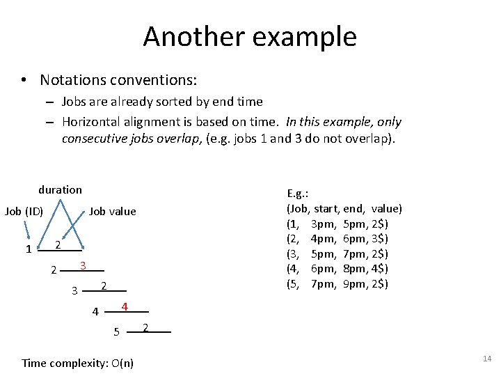
Another example • Notations conventions: – Jobs are already sorted by end time – Horizontal alignment is based on time. In this example, only consecutive jobs overlap, (e. g. jobs 1 and 3 do not overlap). duration Job (ID) 1 E. g. : (Job, start, end, value) (1, 3 pm, 5 pm, 2$) (2, 4 pm, 6 pm, 3$) (3, 5 pm, 7 pm, 2$) (4, 6 pm, 8 pm, 4$) (5, 7 pm, 9 pm, 2$) Job value 2 3 2 2 3 4 4 5 Time complexity: O(n) 2 14

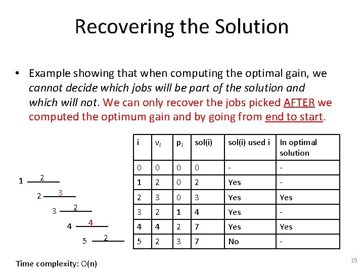
Recovering the Solution • Example showing that when computing the optimal gain, we cannot decide which jobs will be part of the solution and which will not. We can only recover the jobs picked AFTER we computed the optimum gain and by going from end to start. 1 2 3 2 2 3 4 4 5 Time complexity: O(n) 2 i vi pi sol(i) used i In optimal solution 0 0 - - 1 2 0 2 Yes - 2 3 0 3 Yes 3 2 1 4 Yes - 4 4 2 7 Yes 5 2 3 7 No 15

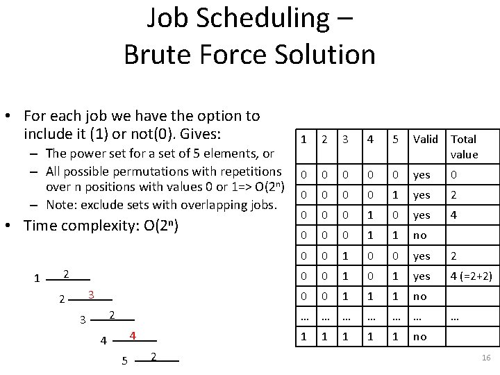
Job Scheduling – Brute Force Solution • For each job we have the option to include it (1) or not(0). Gives: 1 2 3 4 5 Valid Total value 0 0 yes 0 0 1 yes 2 0 0 0 1 0 yes 4 0 0 0 1 1 no 0 0 1 0 0 yes 2 0 0 1 yes 4 (=2+2) 0 0 1 1 1 no … … … 1 1 1 – The power set for a set of 5 elements, or – All possible permutations with repetitions 0 over n positions with values 0 or 1=> O(2 n) 0 – Note: exclude sets with overlapping jobs. • Time complexity: O(2 n) 1 2 3 2 2 3 4 4 5 2 1 1 … no 16

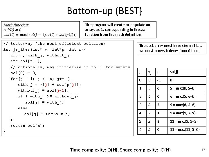
Bottom-up (BEST) The program will create an populate an array, sol, corresponding to the sol function from the math definition. // Bottom-up (the most efficient solution) int js_iter(int* v, int*p, int n){ int j, with_j, without_j; int sol[n+1]; // optionally, may initialize it to -1 for safety sol[0] = 0; for(j = 1; j <= n; j++){ with_j = v[j] + sol[p[j]]; without_j = sol[j-1]; if ( with_j >= without_j) sol[j] = with_j; else sol[j] = without_j; } return sol[n]; } The sol array must have size n+1 b. c. we must access indexes from 0 to n. j vj pj sol[j] 0 0 -1 0 1 5 0 5 = max{0, 5+0} 2 6 0 6 = max{5, 6+0} 3 3 2 9 = max{6, 3+6} 4 2 1 9 = max{9, 2+5} 5 2 3 11 = max{9, 2+9} 6 5 0 11 = max{11, 5+0} Time complexity: Θ(N), Space complexity: Θ(N) 17

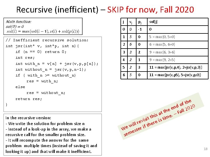
Recursive (inefficient) – SKIP for now, Fall 2020 // Inefficient recursive solution: int jsr(int* v, int*p, int n){ if (n == 0) return 0; int res; int with_n = v[n] + jsr(v, p, p[n]); int without_n = jsr(v, p, n-1); if ( with_n >= without_n) res = with_n; else res = without_n; return res; } In the recursive version: - We write the solution for problem size n - Instead of a look-up in the array, we make a recursive call for the smaller problem size. - It will recompute the answer for the same problem multiple times (instead of saving it and looking it up) and that will make it inefficient. j vj pj sol[j] 0 0 -1 0 1 5 0 5 = max{0, 5+0} 2 6 0 6 = max{5, 6+0} 3 3 2 9 = max{6, 3+6} 4 2 1 9 = max{9, 2+5} 5 2 3 11 = max{jsr(v, p, 4), 2+jsr(v, p, 3)} 6 5 0 11 = max{jsr(v, p 5), 5+jsr(v, p, 0)} he t f o d 20 n 0 e 2 e th – Fall t a his time. t t i is s i v e e r r l e wil r if th e W este sem 18

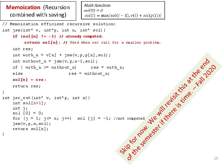
Memoization (Recursion combined with saving) Sk of ip f th or e s no em w es. W te e w r i f t ill r he ev re isi is t t ti hi m s a e. t – th Fa e ll 2 en 02 d 0 // Memoization efficient recursive solution: int jsm(int* v, int*p, int n, int* sol){ if (sol[n] != -1) // already computed. return sol[n]; // Used when rec call for a smaller problem. int res; int with_n = v[n] + jsm(v, p, p[n], sol); int without_n = jsm(v, p, n-1, sol); if ( with_n >= without_n) res = with_n; else res = without_n; sol[n] = res; return res; } int jsr_out(int* v, int*p, int n){ int sol[n+1]; int j; sol [0] = 0; for (j = 1; j<= n; j++) sol [j] = -1; //not computed jsm(v, p, n, sol); return sol[n]; } 19

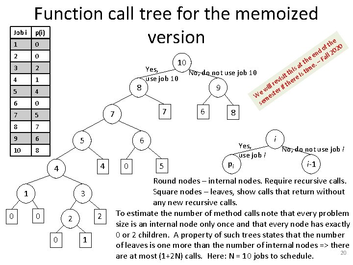
1 Function call tree for the memoized version 2 0 3 2 4 1 5 4 6 0 7 5 8 7 9 6 10 8 Job i p(i) 0 10 8 5 3 0 2 2 0 1 6 8 6 4 1 0 7 7 4 Yes, use job 10 the 0 f d o l 202 n e e Fal h t t e. – a is im No, do not use job 10 th is t t i vis here e r ill r if t 9 w e te W mes se 0 5 pi Yes, use job i i No, do not use job i i-1 Round nodes – internal nodes. Require recursive calls. Square nodes – leaves, show calls that return without any new recursive calls. To estimate the number of method calls note that every problem size is an internal node only once and that every node has exactly 0 or 2 children. A property of such trees states that the number of leaves is one more than the number of internal nodes => there 20 are at most (1+2 N) calls. Here: N = 10 jobs to schedule.

Fibonacci Numbers 21

Fibonacci Numbers • Generate Fibonacci numbers – 3 solutions: inefficient recursive, memoization (top-down dynamic programming (DP)), bottom-up DP. – Not an optimization problem but it has overlapping subproblems => DP eliminates recomputing the same problem over and over again. 22

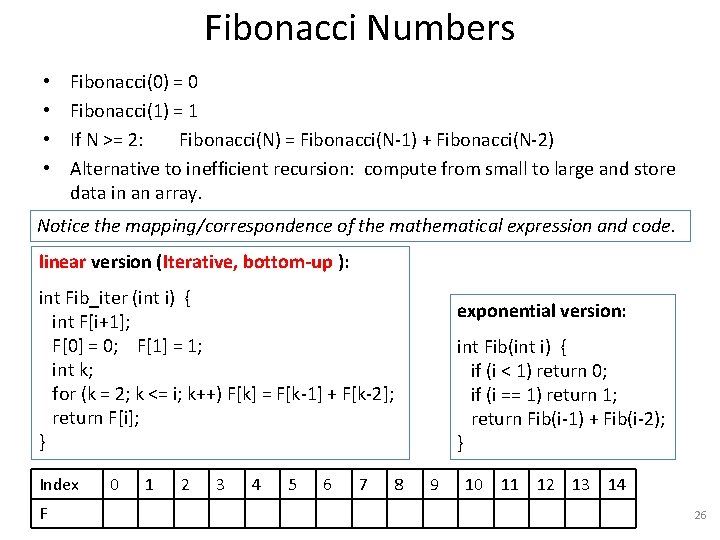
Fibonacci Numbers • Fibonacci(0) = 0 • Fibonacci(1) = 1 • If N >= 2: Fibonacci(N) = Fibonacci(N-1) + Fibonacci(N-2) • How can we write a function that computes Fibonacci numbers? 23

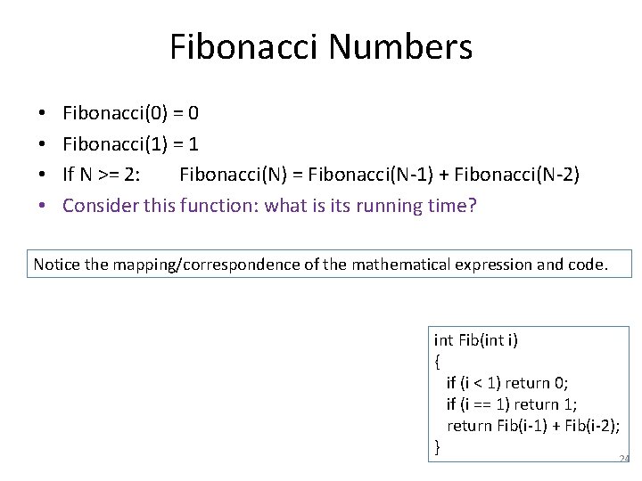
Fibonacci Numbers • • Fibonacci(0) = 0 Fibonacci(1) = 1 If N >= 2: Fibonacci(N) = Fibonacci(N-1) + Fibonacci(N-2) Consider this function: what is its running time? Notice the mapping/correspondence of the mathematical expression and code. int Fib(int i) { if (i < 1) return 0; if (i == 1) return 1; return Fib(i-1) + Fib(i-2); } 24

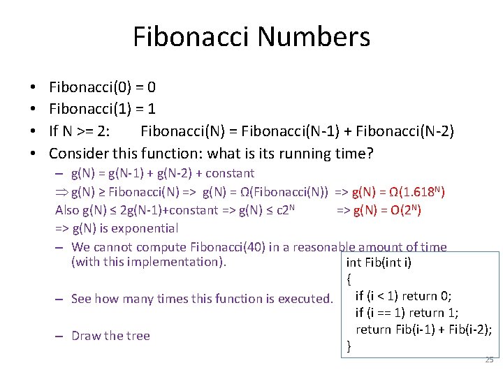
Fibonacci Numbers • • Fibonacci(0) = 0 Fibonacci(1) = 1 If N >= 2: Fibonacci(N) = Fibonacci(N-1) + Fibonacci(N-2) Consider this function: what is its running time? – g(N) = g(N-1) + g(N-2) + constant Þ g(N) ≥ Fibonacci(N) => g(N) = Ω(Fibonacci(N)) => g(N) = Ω(1. 618 N) Also g(N) ≤ 2 g(N-1)+constant => g(N) ≤ c 2 N => g(N) = O(2 N) => g(N) is exponential – We cannot compute Fibonacci(40) in a reasonable amount of time (with this implementation). int Fib(int i) { – See how many times this function is executed. if (i < 1) return 0; if (i == 1) return 1; return Fib(i-1) + Fib(i-2); – Draw the tree } 25

Fibonacci Numbers • • Fibonacci(0) = 0 Fibonacci(1) = 1 If N >= 2: Fibonacci(N) = Fibonacci(N-1) + Fibonacci(N-2) Alternative to inefficient recursion: compute from small to large and store data in an array. Notice the mapping/correspondence of the mathematical expression and code. linear version (Iterative, bottom-up ): int Fib_iter (int i) { int F[i+1]; F[0] = 0; F[1] = 1; int k; for (k = 2; k <= i; k++) F[k] = F[k-1] + F[k-2]; return F[i]; } Index F 0 1 2 3 4 5 6 7 exponential version: int Fib(int i) { if (i < 1) return 0; if (i == 1) return 1; return Fib(i-1) + Fib(i-2); } 8 9 10 11 12 13 14 26

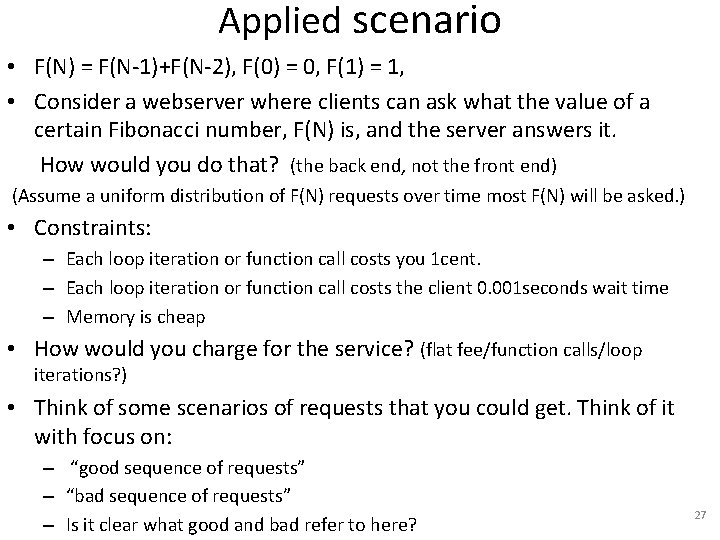
Applied scenario • F(N) = F(N-1)+F(N-2), F(0) = 0, F(1) = 1, • Consider a webserver where clients can ask what the value of a certain Fibonacci number, F(N) is, and the server answers it. How would you do that? (the back end, not the front end) (Assume a uniform distribution of F(N) requests over time most F(N) will be asked. ) • Constraints: – Each loop iteration or function call costs you 1 cent. – Each loop iteration or function call costs the client 0. 001 seconds wait time – Memory is cheap • How would you charge for the service? (flat fee/function calls/loop iterations? ) • Think of some scenarios of requests that you could get. Think of it with focus on: – “good sequence of requests” – “bad sequence of requests” – Is it clear what good and bad refer to here? 27

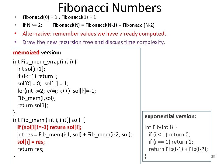
• • Fibonacci Numbers Fibonacci(0) = 0 , Fibonacci(1) = 1 If N >= 2: Fibonacci(N) = Fibonacci(N-1) + Fibonacci(N-2) • Alternative: remember values we have already computed. • Draw the new recursion tree and discuss time complexity. memoized version: int Fib_mem_wrap(int i) { int sol[i+1]; if (i<=1) return i; sol[0] = 0; sol[1] = 1; for(int k=2; k<=i; k++) sol[k]=-1; Fib_mem(i, sol); return sol[i]; } int Fib_mem (int i, int[] sol) { if (sol[i]!=-1) return sol[i]; int res = Fib_mem(i-1, sol) + Fib_mem(i-2, sol); sol[i] = res; return res; } exponential version: int Fib(int i) { if (i < 1) return 0; if (i == 1) return 1; return Fib(i-1) + Fib(i-2); } 28

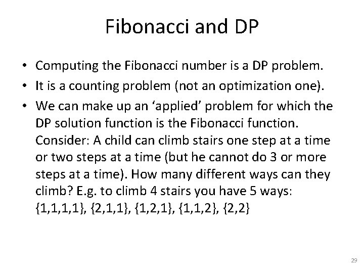
Fibonacci and DP • Computing the Fibonacci number is a DP problem. • It is a counting problem (not an optimization one). • We can make up an ‘applied’ problem for which the DP solution function is the Fibonacci function. Consider: A child can climb stairs one step at a time or two steps at a time (but he cannot do 3 or more steps at a time). How many different ways can they climb? E. g. to climb 4 stairs you have 5 ways: {1, 1, 1, 1}, {2, 1, 1}, {1, 2, 1}, {1, 1, 2}, {2, 2} 29

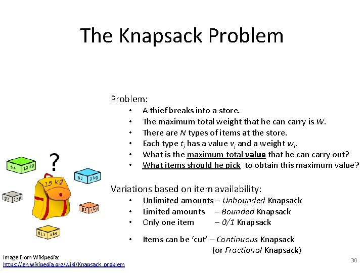
The Knapsack Problem: • • • A thief breaks into a store. The maximum total weight that he can carry is W. There are N types of items at the store. Each type ti has a value vi and a weight wi. What is the maximum total value that he can carry out? What items should he pick to obtain this maximum value? Variations based on item availability: Image from Wikipedia: https: //en. wikipedia. org/wiki/Knapsack_problem • • • Unlimited amounts – Unbounded Knapsack Limited amounts – Bounded Knapsack Only one item – 0/1 Knapsack • Items can be ‘cut’ – Continuous Knapsack (or Fractional Knapsack) 30

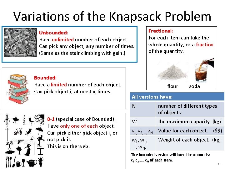
Variations of the Knapsack Problem Unbounded: Have unlimited number of each object. Can pick any object, any number of times. (Same as the stair climbing with gain. ) Bounded: Have a limited number of each object. Can pick object i, at most xi times. 0 -1 (special case of Bounded): Have only one of each object. Can pick either pick object i, or not pick it. This is on the web. Fractional: For each item can take the whole quantity, or a fraction of the quantity. flour soda All versions have: N number of different types of objects W the maximum capacity (kg) v 1, v 2, …, v. N Value for each object. ($$) w 1, …, w. N, Weight of each object. (kg) The bounded version will have the amounts: c 1, c 2, …, c. N of each item. 31

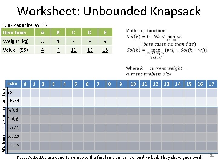
Worksheet: Unbounded Knapsack Max capacity: W=17 Item type: A B C D E Weight (kg) 3 4 7 8 9 Value ($$) 4 6 11 13 15 Work (to compute solution) solution index 0 1 2 3 4 5 6 7 8 9 10 11 12 13 14 15 16 17 Sol Picked A, 3, 4 B, 4, 6 C, 7, 11 D, 8, 13 E, 9, 15 Rows A, B, C, D, E are used to compute the final solution, in Sol and Picked. They show your work. 32

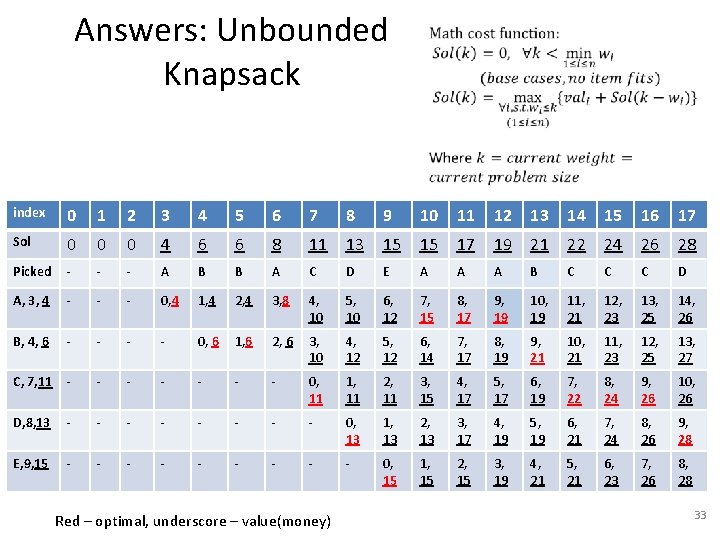
Answers: Unbounded Knapsack index 0 1 2 3 4 5 6 7 8 9 10 11 12 13 14 15 16 17 Sol 0 0 0 4 6 6 8 11 13 15 15 17 19 21 22 24 26 28 Picked - - - A B B A C D E A A A B C C C D A, 3, 4 - - - 0, 4 1, 4 2, 4 3, 8 4, 10 5, 10 6, 12 7, 15 8, 17 9, 19 10, 19 11, 21 12, 23 13, 25 14, 26 B, 4, 6 - - 0, 6 1, 6 2, 6 3, 10 4, 12 5, 12 6, 14 7, 17 8, 19 9, 21 10, 21 11, 23 12, 25 13, 27 C, 7, 11 - - - - 0, 11 1, 11 2, 11 3, 15 4, 17 5, 17 6, 19 7, 22 8, 24 9, 26 10, 26 D, 8, 13 - - - - 0, 13 1, 13 2, 13 3, 17 4, 19 5, 19 6, 7, 21 24 8, 26 9, 28 E, 9, 15 - - - - - 0, 15 1, 15 2, 15 3, 19 4, 21 5, 21 7, 26 8, 28 Red – optimal, underscore – value(money) 6, 23 33

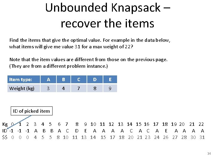
Unbounded Knapsack – recover the items Find the items that give the optimal value. For example in the data below, what items will give me value 31 for a max weight of 22? Note that the item values are different from those on the previous page. (They are from a different problem instance. ) Item type: A B C D E Weight (kg) 3 4 7 8 9 ID of picked item Kg 0 1 2 3 4 5 6 7 8 9 10 11 12 13 14 15 16 17 18 19 20 21 22 ID -1 -1 A B B A C D E A A C A E A A A A $$ 0 0 0 4 5 5 8 10 11 13 14 15 17 18 20 21 23 24 26 27 28 30 31 34

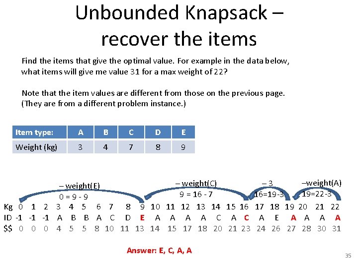
Unbounded Knapsack – recover the items Find the items that give the optimal value. For example in the data below, what items will give me value 31 for a max weight of 22? Note that the item values are different from those on the previous page. (They are from a different problem instance. ) Item type: A B C D E Weight (kg) 3 4 7 8 9 –weight(A) – weight(C) – 3 – weight(E) 19=22 -3 9 = 16 - 7 16=19 -3 0 = 9 - 9 Kg 0 1 2 3 4 5 6 7 8 9 10 11 12 13 14 15 16 17 18 19 20 21 22 ID -1 -1 A B B A C D E A A C A E A A A A $$ 0 0 0 4 5 5 8 10 11 13 14 15 17 18 20 21 23 24 26 27 28 30 31 Answer: E, C, A, A 35

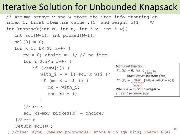
Iterative Solution for Unbounded Knapsack /* Assume arrays v and w store the item info starting at index 1: first item has value v[1] and weight w[1] */ int knapsack(int W, int n, int * v, int * w){ int sol[W+1]; int picked[W+1]; sol[0] = 0; for(k=1; k<=W; k++) { mx = 0; choice = -1; // no item for(i=0; i<n; i++) { if (k>=w[i]) { with_i = v[i]+sol[k-w[i]]; if (mx < with_i) { mx = with_i; choice = i; } }// for i sol[k]=mx; picked[k] = choice; }// for k return sol[W]; } //Time: Θ(n. W) [pseudo polynomial: store W in lg. W bits] Space: Θ(W) 36

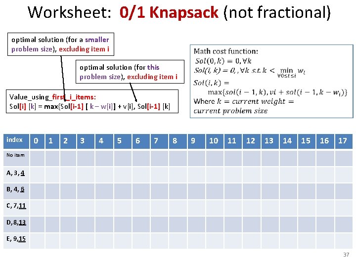
Worksheet: 0/1 Knapsack (not fractional) optimal solution (for a smaller problem size), excluding item i optimal solution (for this problem size), excluding item i Value_using_first_i_items: Sol[i] [k] = max{Sol[i-1] [ k – w[i]] + v[i], Sol[i-1] [k] index 0 1 2 3 4 5 6 7 8 9 10 11 12 13 14 15 16 17 No item A, 3, 4 B, 4, 6 C, 7, 11 D, 8, 13 E, 9, 15 37

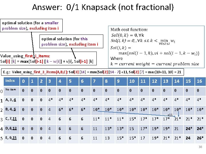
Answer: 0/1 Knapsack (not fractional) optimal solution (for a smaller problem size), excluding item i optimal solution (for this problem size), excluding item i Value_using_first_i_items: Sol[i] [k] = max{Sol[i-1] [ k – w[i]] + v[i], Sol[i-1] [k] E. g. : Value_using_first_3_items(A, B, C): Sol[3] [14] = max{Sol[2] [14 - 7] +11, Sol[2] [7] = max{10+11, 10} = 21 index 0 1 2 3 4 5 6 7 8 9 10 11 12 13 14 15 16 0 No item 0 0 0 0 0 1 A, 3, 4 0 0 0 4* 4* 4* 4* 2 B, 4, 6 0 0 0 4 6* 6* 6* 10* 10* 10* 3 C, 7, 11 0 0 0 4 6 6 6 11* 11* 15* 17* 17* 21* 21* 4 D, 8, 13 0 0 0 4 6 6 6 11 13* 15 5 E, 9, 15 0 0 0 4 6 6 6 11 13 15* 17 +11 17* 19* 21 24* 19* 21* 24 26* 38

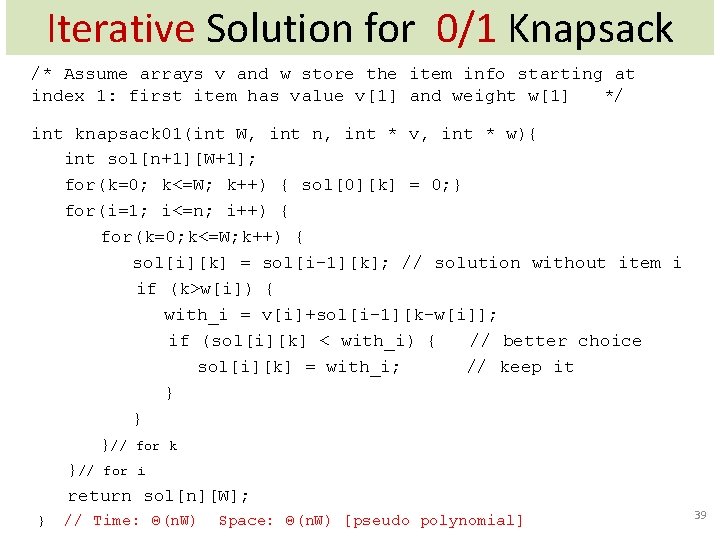
Iterative Solution for 0/1 Knapsack /* Assume arrays v and w store the item info starting at index 1: first item has value v[1] and weight w[1] */ int knapsack 01(int W, int n, int * v, int * w){ int sol[n+1][W+1]; for(k=0; k<=W; k++) { sol[0][k] = 0; } for(i=1; i<=n; i++) { for(k=0; k<=W; k++) { sol[i][k] = sol[i-1][k]; // solution without item i if (k>w[i]) { with_i = v[i]+sol[i-1][k-w[i]]; if (sol[i][k] < with_i) { // better choice sol[i][k] = with_i; // keep it } } }// for k }// for i return sol[n][W]; } // Time: Θ(n. W) Space: Θ(n. W) [pseudo polynomial] 39

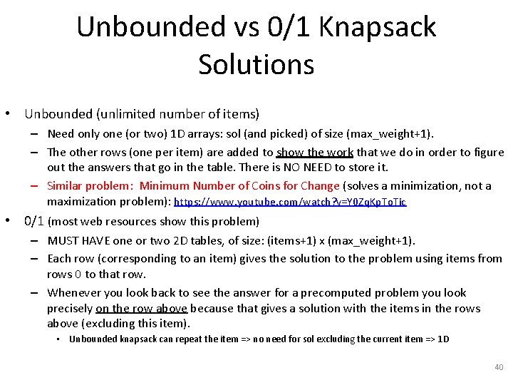
Unbounded vs 0/1 Knapsack Solutions • Unbounded (unlimited number of items) – Need only one (or two) 1 D arrays: sol (and picked) of size (max_weight+1). – The other rows (one per item) are added to show the work that we do in order to figure out the answers that go in the table. There is NO NEED to store it. – Similar problem: Minimum Number of Coins for Change (solves a minimization, not a maximization problem): https: //www. youtube. com/watch? v=Y 0 Zq. Kp. To. Tic • 0/1 (most web resources show this problem) – MUST HAVE one or two 2 D tables, of size: (items+1) x (max_weight+1). – Each row (corresponding to an item) gives the solution to the problem using items from rows 0 to that row. – Whenever you look back to see the answer for a precomputed problem you look precisely on the row above because that gives a solution with the items in the rows above (excluding this item). • Unbounded knapsack can repeat the item => no need for sol excluding the current item => 1 D 40

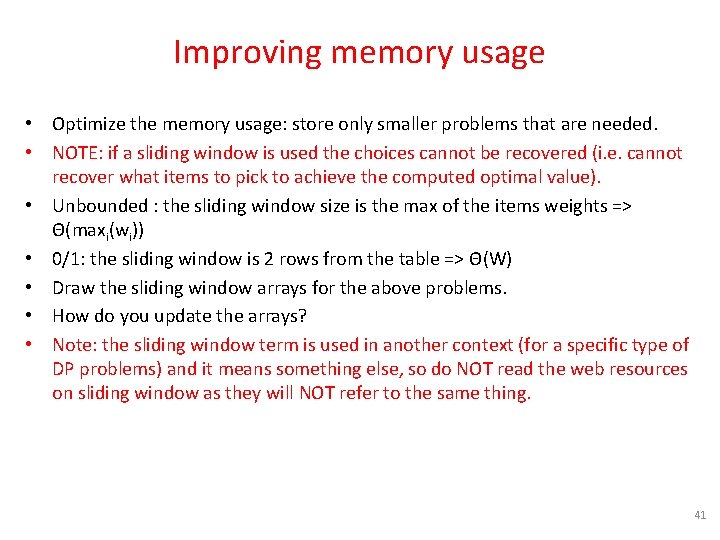
Improving memory usage • Optimize the memory usage: store only smaller problems that are needed. • NOTE: if a sliding window is used the choices cannot be recovered (i. e. cannot recover what items to pick to achieve the computed optimal value). • Unbounded : the sliding window size is the max of the items weights => Θ(maxi(wi)) • 0/1: the sliding window is 2 rows from the table => Θ(W) • Draw the sliding window arrays for the above problems. • How do you update the arrays? • Note: the sliding window term is used in another context (for a specific type of DP problems) and it means something else, so do NOT read the web resources on sliding window as they will NOT refer to the same thing. 41

Hint for DP problems • For a DP problem you can typically write a MATH function that gives the solution for problem of size N in terms of smaller problems. • It is straightforward to go from this math function to code: – Iterative: The math function ‘maps’ to the sol array – Recursive: The math function ‘maps’ to recursive calls • Typically the math function will be a – Min/max (over itself applied to smaller N) – Sum (over itself applied to smaller N) 42

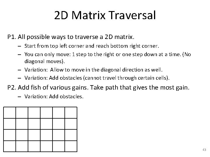
2 D Matrix Traversal P 1. All possible ways to traverse a 2 D matrix. – Start from top left corner and reach bottom right corner. – You can only move: 1 step to the right or one step down at a time. (No diagonal moves). – Variation: Allow to move in the diagonal direction as well. – Variation: Add obstacles (cannot travel through certain cells). P 2. Add fish of various gains. Take path that gives the most gain. – Variation: Add obstacles. 43

Longest Common Subsequence (LCS) 44

Longest Common Subsequence (LCS) • Given 2 sequences, find the longest common subsequence (LCS) • Example: – A B C B D A B – B D C A B A • Examples of subsequences of the above sequences: – – – BCBA (length 4) BDAB CBA (length 3) CAB BB (length 2) Show the components of the solution. Can you show a solution similar that of an Edit distance problem? 45

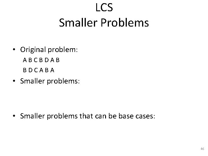
LCS Smaller Problems • Original problem: A B C B D A B B D C A B A • Smaller problems: • Smaller problems that can be base cases: 46

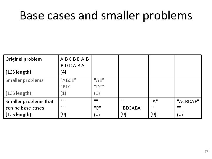
Base cases and smaller problems Original problem (LCS length) Smaller problems A B C B D A B B D C A B A (4) (LCS length) "ABCB" "BD" (1) "AB" "DC" (0) Smaller problems that can be base cases (LCS length) "" "" (0) "" "BDCABA" (0) "A" "" (0) "ACBDAB" "" (0) 47

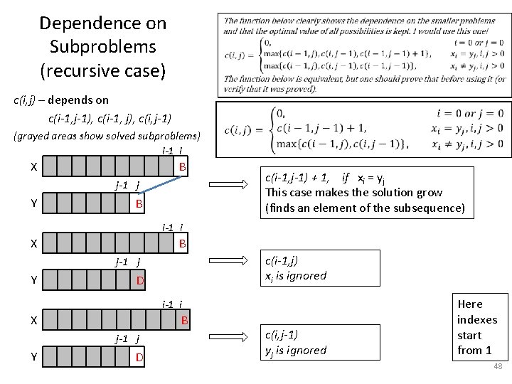
Dependence on Subproblems (recursive case) c(i, j) – depends on c(i-1, j-1), c(i-1, j), c(i, j-1) (grayed areas show solved subproblems) i-1 i B X j-1 j Y B c(i-1, j-1) + 1, if xi = yj This case makes the solution grow (finds an element of the subsequence) i-1 i B X c(i-1, j) xi is ignored j-1 j Y D i-1 i B X j-1 j Y D c(i, j-1) yj is ignored Here indexes start from 1 48

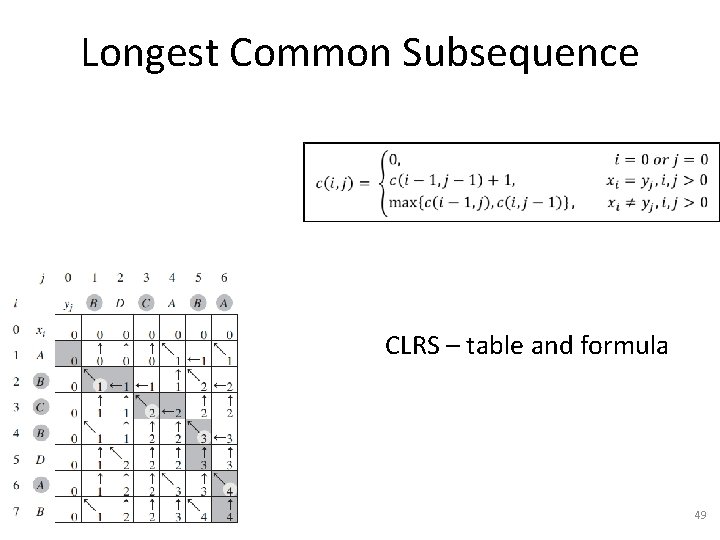
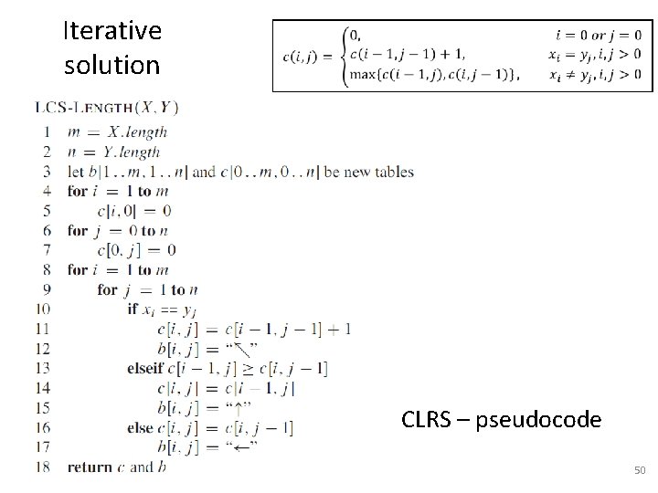
Longest Common Subsequence CLRS – table and formula 49

Iterative solution CLRS – pseudocode 50

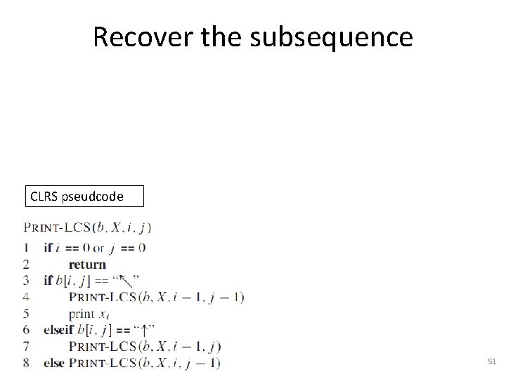
Recover the subsequence CLRS pseudcode 51

Longest Increasing Subsequence (LIS) 52

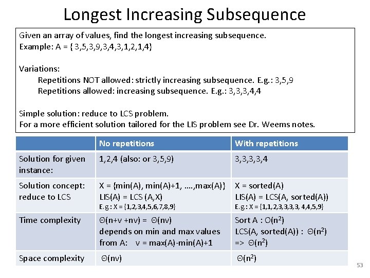
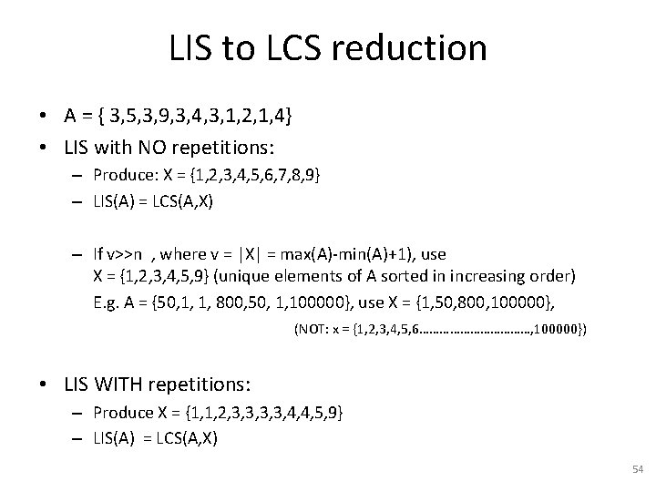
Longest Increasing Subsequence Given an array of values, find the longest increasing subsequence. Example: A = { 3, 5, 3, 9, 3, 4, 3, 1, 2, 1, 4} Variations: Repetitions NOT allowed: strictly increasing subsequence. E. g. : 3, 5, 9 Repetitions allowed: increasing subsequence. E. g. : 3, 3, 3, 4, 4 Simple solution: reduce to LCS problem. For a more efficient solution tailored for the LIS problem see Dr. Weems notes. No repetitions With repetitions Solution for given instance: 1, 2, 4 (also: or 3, 5, 9) 3, 3, 4 Solution concept: reduce to LCS X = {min(A), min(A)+1, …. , max(A)} LIS(A) = LCS (A, X) X = sorted(A) LIS(A) = LCS(A, sorted(A)) Time complexity Θ(n+v +nv) = Θ(nv) depends on min and max values from A: v = max(A)-min(A)+1 Sort A : O(n 2) LCS(A, sorted(A)) : Θ(n 2) => Θ(n 2) Space complexity Θ(nv) Θ(n 2) E. g. : X = {1, 2, 3, 4, 5, 6, 7, 8, 9} E. g. : X = {1, 1, 2, 3, 3, 4, 4, 5, 9} 53

LIS to LCS reduction • A = { 3, 5, 3, 9, 3, 4, 3, 1, 2, 1, 4} • LIS with NO repetitions: – Produce: X = {1, 2, 3, 4, 5, 6, 7, 8, 9} – LIS(A) = LCS(A, X) – If v>>n , where v = |X| = max(A)-min(A)+1), use X = {1, 2, 3, 4, 5, 9} (unique elements of A sorted in increasing order) E. g. A = {50, 1, 1, 800, 50, 1, 100000}, use X = {1, 50, 800, 100000}, (NOT: x = {1, 2, 3, 4, 5, 6………………, 100000}) • LIS WITH repetitions: – Produce X = {1, 1, 2, 3, 3, 4, 4, 5, 9} – LIS(A) = LCS(A, X) 54

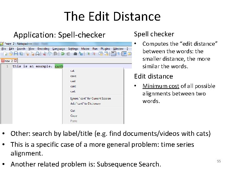
The Edit Distance Application: Spell-checker Spell checker • Computes the “edit distance” between the words: the smaller distance, the more similar the words. Edit distance • Minimum cost of all possible alignments between two words. • Other: search by label/title (e. g. find documents/videos with cats) • This is a specific case of a more general problem: time series alignment. • Another related problem is: Subsequence Search. 55

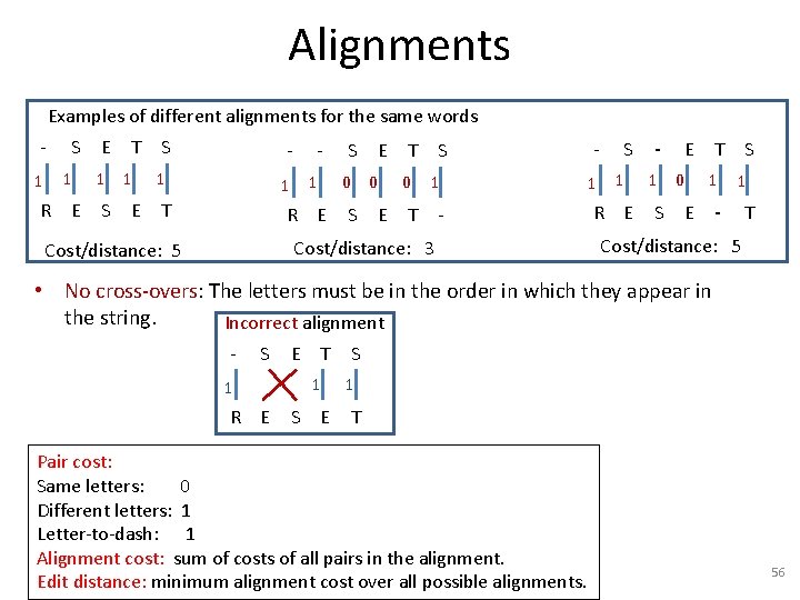
Alignments Examples of different alignments for the same words 1 S 1 R E E T S - - 1 1 1 S T E R E S E T 0 0 0 S T E S 1 - Cost/distance: 3 Cost/distance: 5 1 S 1 R E - E T 1 0 1 S - E S 1 T Cost/distance: 5 • No cross-overs: The letters must be in the order in which they appear in the string. Incorrect alignment - S E T 1 1 R E S 1 T Pair cost: Same letters: 0 Different letters: 1 Letter-to-dash: 1 Alignment cost: sum of costs of all pairs in the alignment. Edit distance: minimum alignment cost over all possible alignments. 56

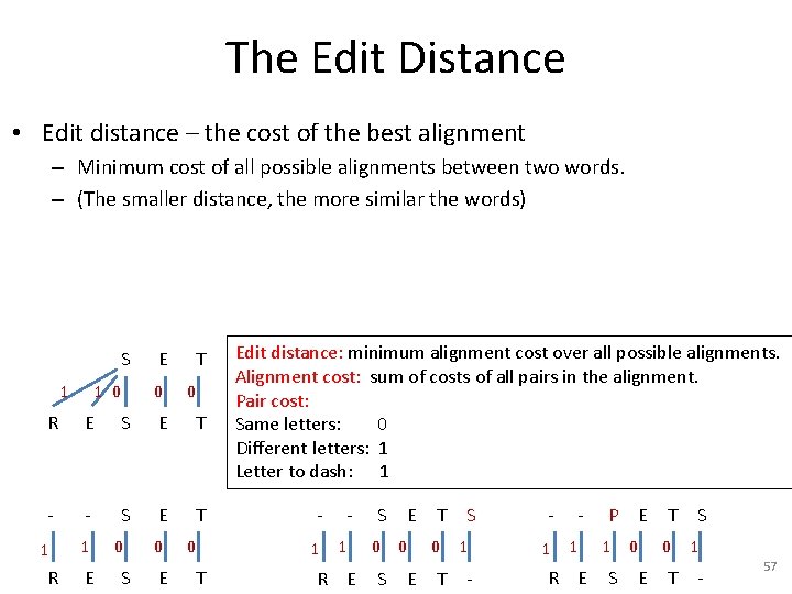
The Edit Distance • Edit distance – the cost of the best alignment – Minimum cost of all possible alignments between two words. – (The smaller distance, the more similar the words) S 1 1 0 E 0 T 0 R E S E T - - S E T 1 1 R E 0 S 0 E 0 T Edit distance: minimum alignment cost over all possible alignments. Alignment cost: sum of costs of all pairs in the alignment. Pair cost: Same letters: 0 Different letters: 1 Letter to dash: 1 - - 1 1 R E S E T 0 0 0 S T E S 1 - - - 1 1 R E P E T 1 0 0 S T E S 1 - 57

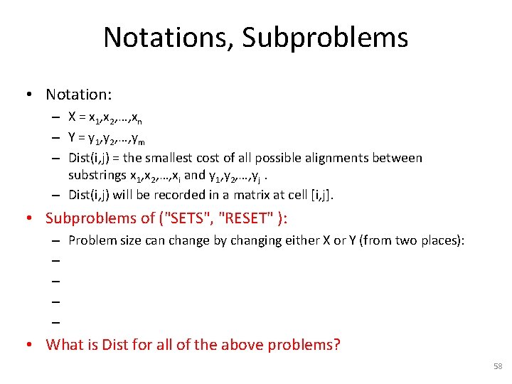
Notations, Subproblems • Notation: – X = x 1, x 2, …, xn – Y = y 1, y 2, …, ym – Dist(i, j) = the smallest cost of all possible alignments between substrings x 1, x 2, …, xi and y 1, y 2, …, yj. – Dist(i, j) will be recorded in a matrix at cell [i, j]. • Subproblems of ("SETS", "RESET" ): – – – Problem size can change by changing either X or Y (from two places): • What is Dist for all of the above problems? 58

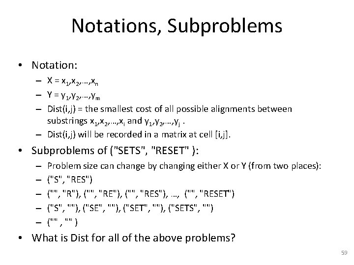
Notations, Subproblems • Notation: – X = x 1, x 2, …, xn – Y = y 1, y 2, …, ym – Dist(i, j) = the smallest cost of all possible alignments between substrings x 1, x 2, …, xi and y 1, y 2, …, yj. – Dist(i, j) will be recorded in a matrix at cell [i, j]. • Subproblems of ("SETS", "RESET" ): – – – Problem size can change by changing either X or Y (from two places): ("S", "RES") ("", "R"), ("", "RES"), …, ("", "RESET") ("S", ""), ("SET", ""), ("SETS", "") ("" , "" ) • What is Dist for all of the above problems? 59

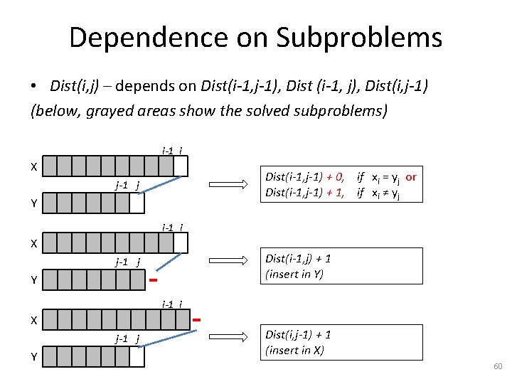
Dependence on Subproblems • Dist(i, j) – depends on Dist(i-1, j-1), Dist (i-1, j), Dist(i, j-1) (below, grayed areas show the solved subproblems) i-1 i X Dist(i-1, j-1) + 0, if xi = yj or Dist(i-1, j-1) + 1, if xi ≠ yj j-1 j Y i-1 i X Dist(i-1, j) + 1 (insert in Y) j-1 j Y i-1 i X j-1 j Y Dist(i, j-1) + 1 (insert in X) 60

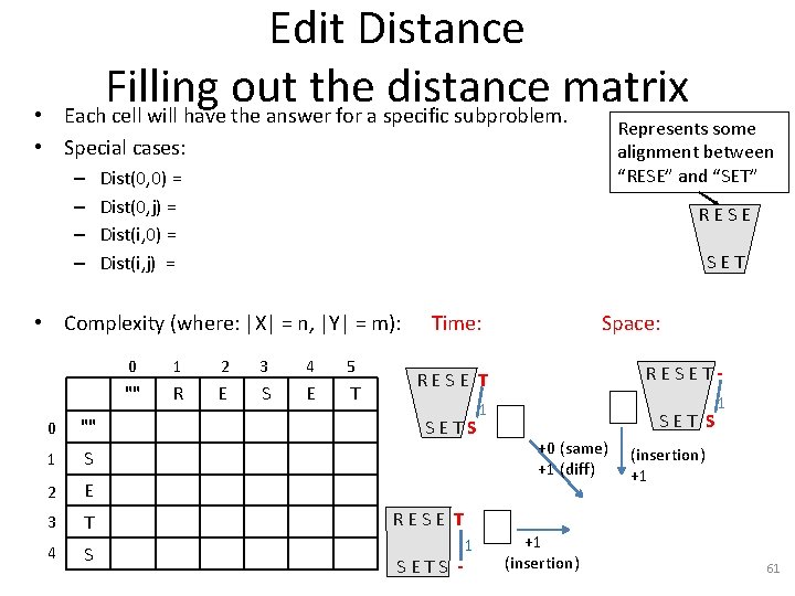
Edit Distance Filling out the distance matrix Each cell will have the answer for a specific subproblem. • • Special cases: Represents some alignment between “RESE” and “SET” – Dist(0, 0) = – Dist(0, j) = – Dist(i, 0) = – Dist(i, j) = R E S E T • Complexity (where: |X| = n, |Y| = m): Time: Space: 0 "" 1 S 2 E 3 T 4 S 0 1 2 3 4 5 "" R E S E T 1 S E T S R E S E T S +0 (same) +1 (diff) 1 (insertion) +1 R E S E T S - 1 +1 (insertion) 61

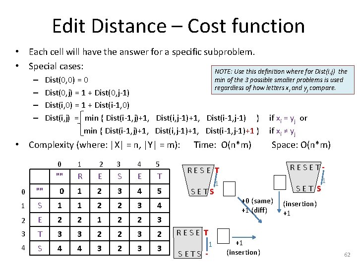
Edit Distance – Cost function • Each cell will have the answer for a specific subproblem. • Special cases: NOTE: Use this definition where for Dist(i, j) the min of the 3 possible smaller problems is used regardless of how letters xi and yj compare. – Dist(0, 0) = 0 – Dist(0, j) = 1 + Dist(0, j-1) – Dist(i, 0) = 1 + Dist(i-1, 0) – Dist(i, j) = min { Dist(i-1, j)+1, Dist(i, j-1)+1, Dist(i-1, j-1) } if xi = yj or min { Dist(i-1, j)+1, Dist(i, j-1)+1, Dist(i-1, j-1)+1 } if xi ≠ yj • Complexity (where: |X| = n, |Y| = m): Time: O(n*m) Space: O(n*m) 0 1 2 3 4 5 "" R E S E T 0 "" 0 1 2 3 4 5 1 S 1 1 2 2 3 4 2 E 2 2 1 2 2 3 3 T 3 3 2 2 3 2 4 S 4 4 3 2 3 3 R E S E T 1 S E T S R E S E T S +0 (same) +1 (diff) 1 (insertion) +1 R E S E T S - 1 +1 (insertion) 62

Edit Distance Sliding Window • Space complexity improvement – Θ(min{|X|, |Y|}) – Keep only two rows – Keep only one row 63

Motivation for Edit Distance • The Edit Distance essentially does Time Series Alignment • Other examples of problems solved with Time Series Alignment: – Given observed temperatures, find location: • Collected in a database temperatures at different hours over one day in various places (labelled with the name). Given a query consisting of temperatures collected in an unknown place, find the place with the most similar temperatures. Issues: – Not same number of measurements for every place and query. – Not at the exact same time. (E. g. maybe Mary recorded more temperatures throughout the day and none in the night, and John collected uniformly throughout the day and night. ) – Find videos showing a similar sign – Find shapes in images (after image processing extracted relevant features) • Find a substring in a string – E. g. swear words in Pokemon Names – Uses two additional sink states (at the beginning and end of the small query) 64

Other DP Problems • • • Rod cutting Stair climbing Make amount with smallest number of coins Matrix with gain House robber Many more on leetcode. 65

Application of the Knapsack problem • https: //en. wikipedia. org/wiki/Knapsack_problem One early application of knapsack algorithms was in the construction and scoring of tests in which the test-takers have a choice as to which questions they answer. For small examples, it is a fairly simple process to provide the test-takers with such a choice. For example, if an exam contains 12 questions each worth 10 points, the testtaker need only answer 10 questions to achieve a maximum possible score of 100 points. However, on tests with a heterogeneous distribution of point values, it is more difficult to provide choices. Feuerman and Weiss proposed a system in which students are given a heterogeneous test with a total of 125 possible points. The students are asked to answer all of the questions to the best of their abilities. Of the possible subsets of problems whose total point values add up to 100, a knapsack algorithm would determine which subset gives each student the highest possible score 66

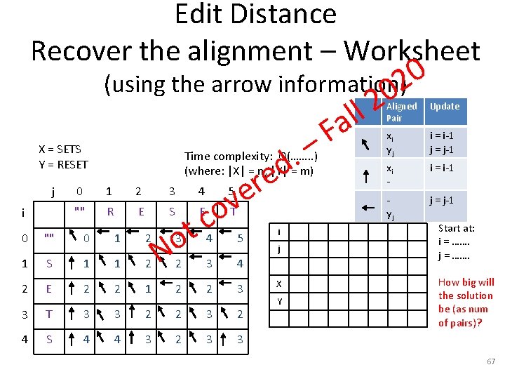
Edit Distance Recover the alignment – Worksheet 0 (using the arrow information) 2 0 X = SETS Y = RESET j i – . d e r e v o Time complexity: O(……. . ) (where: |X| = n, |Y| = m) 0 1 2 3 4 "" R E S E 0 "" 0 1 2 1 S 1 1 2 2 E 2 2 3 T 3 4 S 4 c t o 5 T 3 4 2 3 4 1 2 2 3 3 2 2 3 2 4 3 2 3 3 N a F 5 i j X Y 2 ll Aligned Pair Update xi yj i = i-1 j = j-1 xi - i = i-1 - yj j = j-1 Start at: i = ……. j = ……. How big will the solution be (as num of pairs)? 67

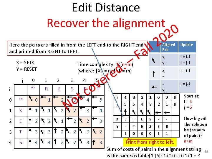
Edit Distance Recover the alignment Here the pairs are filled in from the LEFT end to the RIGHT end and printed from RIGHT to LEFT. X = SETS Y = RESET j i 0 1 2 3 4 "" R E S E 0 "" 0 1 2 1 S 1 1 2 2 E 2 2 3 T 3 4 S 4 c t o 5 T 3 4 2 3 4 1 2 2 3 3 2 2 3 2 4 3 2 3 3 N 5 Aligned Pair Update xi yj i = i-1 j = j-1 xi - i = i-1 - yj j = j-1 2 ll a F – . d e r e v o Time complexity: O(n+m) (where: |X| = n, |Y| = m) 0 2 0 i 4 3 2 1 0 0 0 j 5 5 4 3 2 1 0 X S T E S - - Y - T E S E R 1 0 0 0 1 1 Start at: i = 4 j = 5 How big will the solution be (as num of pairs)? n+m Print from right to left. Sum of costs of pairs in the alignment string is the same as table[4][5]: 1+0+0+0+1+1 = 3 68

• What is the best alignment between abcdefghijk cd. XYZefgh 69

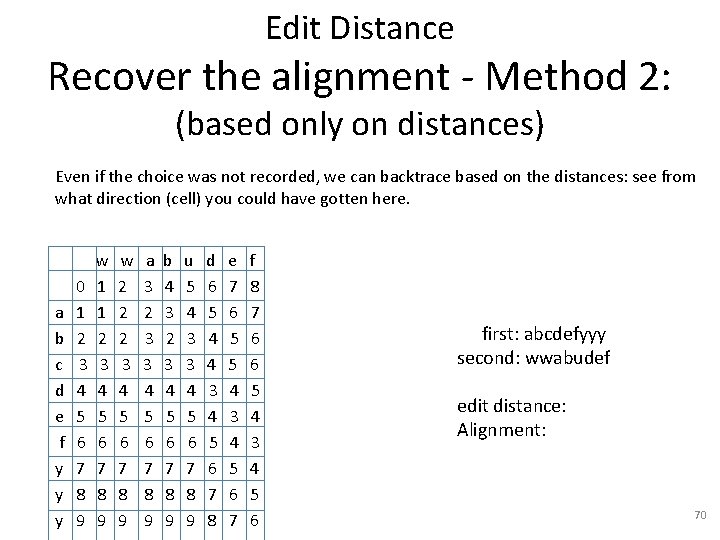
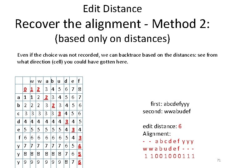
Edit Distance Recover the alignment - Method 2: (based only on distances) Even if the choice was not recorded, we can backtrace based on the distances: see from what direction (cell) you could have gotten here. w w a b u d e f 0 1 2 3 4 5 6 7 8 a 1 1 2 2 3 4 5 6 7 b 2 2 2 3 4 5 6 c 3 3 3 4 5 6 d 4 4 4 3 4 5 e 5 5 5 4 3 4 f 6 6 6 5 4 3 y 7 7 7 6 5 4 y 8 8 8 7 6 5 y 9 9 9 8 7 6 first: abcdefyyy second: wwabudef edit distance: Alignment: 70

Edit Distance Recover the alignment - Method 2: (based only on distances) Even if the choice was not recorded, we can backtrace based on the distances: see from what direction (cell) you could have gotten here. w w a b u d e f 0 1 2 3 4 5 6 7 8 a 1 1 2 2 3 4 5 6 7 b 2 2 2 3 4 5 6 c 3 3 3 4 5 6 d 4 4 4 3 4 5 e 5 5 5 4 3 4 f 6 6 6 5 4 3 y 7 7 7 6 5 4 y 8 8 8 7 6 5 y 9 9 9 8 7 6 first: abcdefyyy second: wwabudef edit distance: 6 Alignment: - - a b c d e f y y y w w a b u d e f - - 1 1 0 0 0 1 1 1 71

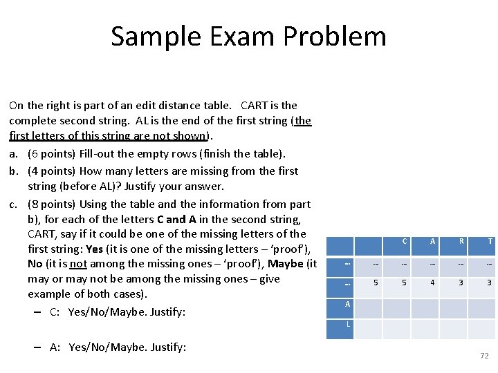
Sample Exam Problem On the right is part of an edit distance table. CART is the complete second string. AL is the end of the first string (the first letters of this string are not shown). a. (6 points) Fill-out the empty rows (finish the table). b. (4 points) How many letters are missing from the first string (before AL)? Justify your answer. c. (8 points) Using the table and the information from part b), for each of the letters C and A in the second string, CART, say if it could be one of the missing letters of the first string: Yes (it is one of the missing letters – ‘proof’), No (it is not among the missing ones – ‘proof’), Maybe (it may or may not be among the missing ones – give example of both cases). – C: Yes/No/Maybe. Justify: – A: Yes/No/Maybe. Justify: C A R T … … … … 5 5 4 3 3 A L 72